Download
1 / 85
990 likes | 1.64k Views
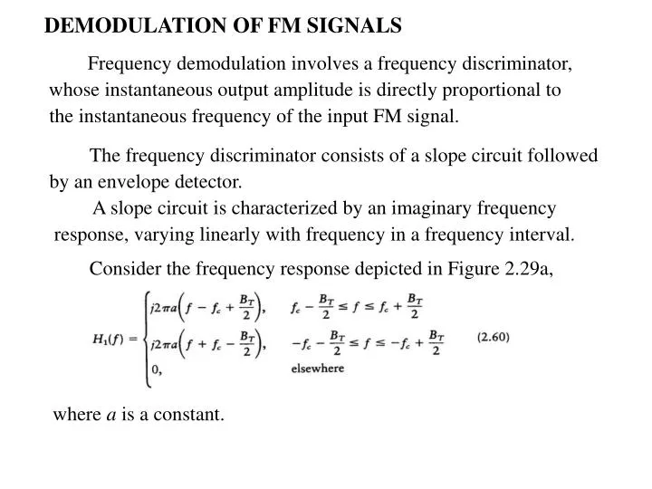
DEMODULATION OF FM SIGNALS Frequency demodulation involves a frequency discriminator, whose instantaneous output amplitude is directly proportional to the instantaneous frequency of the input FM signal. The frequency discriminator consists of a slope circuit followed

E N D
DEMODULATION OF FM SIGNALS Frequency demodulation involves a frequency discriminator, whose instantaneous output amplitude is directly proportional to the instantaneous frequency of the input FM signal. The frequency discriminator consists of a slope circuit followed by an envelope detector. A slope circuit is characterized by an imaginary frequency response, varying linearly with frequency in a frequency interval. Consider the frequency response depicted in Figure 2.29a, where a is a constant.
The response s1(t) of the slope circuit is produced by FM signal s(t) of carrier frequency fc and transmission bandwidth BT. The spectrum of s(t) is essentially zero outside the frequency interval fc - BT/2 < | f | <fc+BT/2. We may replace the BPF with frequency response H1(f) with equivalent LPF with frequency response H1(f) by doing two things: 1). Shifting H1(f) to the right by fc, where fc is the mid-band frequency of the BPF; this operation aligns the translated frequency response of the equivalent LPF with that of the BPF. 2). Seting H1(f)(f - fc) equal to 2H1(f) for f > 0. Thus for the problem at hand we get
Hence, using Eqs. (2.60) and (2.61), we get which is plotted in Figure 1.19b. The incoming FM signal s(t) is defined by Equ. (2.26) : Given that the carrier frequency fc is high compared to the transmission bandwidth of the FM signal s(t), the complex envelope of s(t) is
Let s1(t) denote the complex envelope of the response of the slope circuit defined by Figure 2.29a due to s(t). The Fourier transform of s1(t) can be expressed as: where S(f) is the Fourier transform of s(t).
Multiplication of the Fourier transform of a signal by j2pf is equivalent to differentiating the signal in the time domain. From Equ. (2.64) we deduce Substituting Equ. (2.63) into (2.65), we get The desired response of the slope circuit is therefore
Figure 2.29(a) Frequency response of ideal slope circuit. (b) Frequency response of the slope circuit’s complex low-pass equivalent. (c) Frequency response of the ideal slope circuit complementary to that of part (a).
Provided that we choose we may use an envelope detector to recover the amplitude variations and thus obtain the original message signal. The resulting envelope-detector output is therefore The bias term pBTaAc in Equ. (2.68) may be subtracted from the envelope-detector output |~s1(t)|, the output of a 2nd envelope detector preceded by the complementary slope circuit with a frequency response H2(f) as described in Figure 2.29c. That is, the two slope circuits are related by
Denote s2(t) the response of complementary slope circuit produced by the incoming FM signal s(t). Following similar procedure, we may write where ~s2(t) is the complex envelope of s2(t). Difference between envelopes in Eqs. (2.68) and (2.70) is a scaled version of message signal m(t) and free from bias. Model the frequency discriminator as pair of slope circuits with complex transfer functions related by Equ. (2.69), followed by envelope detectors and a summer, as in Figure 2.30. This scheme is called a balanced frequency discriminator.
FM STEREO MULTIPLEXING Specifications for FM stereo transmission is influenced by : 1). Transmission has to operate within the allocated FM channels. 2). It has to be compatible with monophonic radio receivers. Figure 2.31a shows the block diagram of the multiplexing system used in an FM stereo transmitter. Let mL(t) and mR(t) denote the signals picked up by left-hand and right-hand microphones at the transmitting end of the system. They are applied to a simple matrixer that generates the sum signal, mL(t) + mR(t), and the difference signal, mL(t) - mR(t). The sum signal is left in its baseband form; it is available for monophonic reception. The difference signal and a 38-kHz subcarrier (derived from a 19-kHz crystal oscillator by frequency doubling) are applied to a product modulator, thereby producing a DSB-SC wave.
The multiplexed signal m(t) also includes a 19-kHz pilot to provide reference for coherent detection of the difference signal at the stereo receiver. The multiplexed signal is described by where fc = 19 kHz, and K is the amplitude of the pilot tone. This multiplexed signal m(t) then frequency-modulates the main carrier to produce the transmitted signal.
Figure 2.31(a) Multiplexer in FM stereo. (b) Demultiplexer in FM stereo.
At a stereo receiver, the multiplexed signal m(t) is recovered by frequency demodulating the incoming FM wave. Then m(t) is applied to the demultiplexing system shown in Figure 2.31b. The individual components of the multiplexed signal m(t) are separated by three appropriate filters.
The recovered pilot (using a narrowband filter tuned to 19-kHz) is frequency doubled to produce the desired 38-kHz subcarrier. This subcarrier enables the coherent detection of the DSB-SC modulated wave, thereby recovering the difference signal, mL(t) - mR(t). The baseband LPF in the top path of Figure 2.31b is designed to pass the sum signal, mL(t) + mR(t). Finally, the simple matrixer reconstructs the left-hand signal mL(t) and right-hand signal mR(t), and applies them to their respective speakers.
2.8 Superheterodywe Receiver Besides demodulating, the receiver also performing : • Carrier tuning,to select the desired signal (desired radio or TV station). • Filtering, to separate the desired signal from other modulated signals. • Amplification, to compensate for the loss of signal power. The receiver consists of an RF section, a mixer and LO, an IF section, demodulator, and power amplifier. Typical parameters of commercial AM and FM radio receivers are listed in Table 2.3. Figure 2.32 shows a super-heterodyne receiver for AM using envelope detector for demodulation. The combination of mixer and LO provides heterodyning, whereby the incoming signal is converted to a predetermined IF, usually lower than the incoming carrier frequency.
The heterodyning is to produce an IF carrier defined by fIF = fLO – fRF (2.78) where fLO is the LO frequency and fRF is the RF carrier frequency. The IF section consists of one or more stages of tuned amplification, with a bandwidth corresponding to that required for the particular type of modulation that the receiver is intended to handle. The IF section provides most of the amplification and selectivity in the receiver. The output of the IF section is applied to a demodulator to recover the baseband signal. If coherent detection is used, then a coherent signal source must be provided in the receiver.
In superheterodyne receiver, input frequencies | fLO ± fIF | will result in fIF at the mixer output. This introduces possible simultaneous reception of two signals differing in frequency by twice the fIF. For example, a receiver tuned to 650 kHz and having fIF = 455 kHz is subject to an image interference at 1.56 MHz; any receiver with this fIF, is subject to image interference at a frequency of 910 kHz higher than the desired station. The mixer is incapable of distinguishing between the desired signal and its image in that it produces an IF output from either one of them. The practical cure for image interference is to employ highly selective stages in the RF section to favor the desired signal and discriminate against the image signal.
The basic difference between AM and FM superheterodyne receivers lies in the use of an FM demodulator such as limiter- frequency discriminator. In an FM system, the message information is transmitted by variations of the instantaneous frequency of a sinusoidal carrier, and its amplitude is maintained constant. An amplitude limiter, following the IF section, is used to remove amplitude variations by clipping the modulated wave at the IF section output. The resulting rectangular wave is rounded off by a BPF that suppresses harmonics of the carrier frequency. Thus the filter output is again sinusoidal, with an amplitude that is independent of the carrier amplitude at the receiver input.
Figure 2.32Basic elements of an AM radio receiver of the superheterodyne type.
2.9 Noise in CW Modulation Systems 1). Channel model, which assumes a communication channel that is distortionless but perturbed by additive white Gaussian noise (AWGN). 2). Receiver model, which assumes a receiver consisting of an ideal BPF followed by an ideal demodulator; the BPF is used to minimize the effect of channel noise. Figure 2.33 shows the noisy receiver model that combines the above two assumptions. In this figure, s(t) denotes the incoming modulated signal and w(t) denotes the channel noise. The BPF in Figure 2.33 represents the combined filtering of the tuned amplifiers used in the actual receiver for the signal amplification prior to demodulation.
SIGNAL-TO-NOISE RATIOS: BASIC DEFINITIONS Let the power spectral density (psd) of the noise w(t) be N0/2, N0 being the average noise power per unit bandwidth of the receiver. the receiver BPF in Figure 2.33. For DSB-SC, AM, and FM, with midband frequency of the receiver BPF in Figure 2.33 to be the carrier frequency fc, we may model psd SN(f) of noise n(t), resulting from white noise w(t) through the filter, as shown in Figure 2.34. Typically, fc >> BT , the filtered noise n(t) can be represented as a narrowband noise in the canonical form n(t) = nI(t)cos(2pfct) – nQ(t)sin(2pfct) (2.79) nI(t) : the in-phase noise component, nQ(t) : the quadrature noise component, measured with respect to the carrier wave Accos(2pfct).
The filtered signal x(t) available for demodulation is x(t) = s(t) + n(t) (2.80) The details of s(t) depend on the type of modulation used. The average noise power at the demodulator input is equal to the total area under the curve of the psd SN(f). From Figure 2.34, this average noise power is equal to N0BT. With the demodulated signal s(t) and the filtered noise n(t) appearing additively at the demodulator input (Equ. (2.80)), we may define (SNR)I as the ratio of the average power of the modulated signal s(t) to the average power of the filtered noise n(t). A useful measure of noise performance is the (SNR)O , the ratio of the average power of the demodulated message signal to the average power of the noise, both measured at the receiver output.
Figure 2.34Idealized characteristic of band-pass filtered noise.
When the receiver uses envelope detection as in AM or frequency discrimination as in FM, the average power of the filtered noise n(t) is relatively low to justify the output SNR as a measure of receiver performance. For output SNRC comparison of different modulation- demodulation systems, it must be made on an equal basis: • The modulated signal s(t) transmitted by each system has the same average power. • The channel noise w(t) has the same average power measured in the message bandwidth W.
As a frame of reference we define the channel (SNR)C as the ratio of the average power of the modulated signal to the average power of channel noise in the message bandwidth, both measured at the receiver input. This definition is illustrated in Figure 2.35. We define a figure of merit for the receiver as follows: Figure of merit = (SNR)O/(SNR)C (2.81) The higher the figure of merit, the better the noise performance of the receiver. The figure of merit may = 1, < 1, or > 1, depending on the type of modulation used.
Figure 2.35The baseband transmission model, assuming a message bandwidth Wfor calculating the channel SNR.
2.10 Noise in Linear Receivers Using Coherent Detection AM demodulation depends on whether the carrier is suppressed or not. When the carrier is suppressed we require the use of coherent detection, in which case the receiver is linear. When AM includes transmission of the carrier, demodulation is accomplished by using an envelope detector, in which case the receiver is nonlinear. Figure 2.36 shows the model of a DSB-SC receiver by using a coherent detector. Coherent detection requires multiplication of the filtered signal x(t) by a locally generated cos(2pfct) and then low-pass filtering the product. The DSB-SC component of the filtered signal x(t) is s(t) = CAccos(2pfct) m(t) (2.82) where Accos(2pfct) is the carrier wave and m(t) is the message signal.
In Equ. (2.82), we assume that m(t) is the sample function of a zero mean stationary process, whose psd SM(f) is limited to the message bandwidth W. The average power P of the message signal is the total area under the curve of the psd, as shown by The carrier wave is statistically independent of the message signal. The average power of the DSB-SC modulated signal s(t) may be expressed as C2A2P/2. With a noise spectral density of No/2, the average noise power in the message bandwidth W is equal to WNo. The channel SNR of the DSB-SC system is therefore (SNR)C,DSB = C2Ac2P/2WNo (2.84)
Using the narrowband representation of the filtered noise n(t), the total signal at the coherent detector input may be expressed as where nI(t) and nQ(t) are the in-phase and quadrature components of n(t) with respect to the carrier. The output of the product-modulator component of the coherent detector is The LPF in the coherent detector in Figure 2.36 removes the high-frequency components of v(t), yielding the receiver output
Equ. (2.86) indicates the following: 1). The message signal m(t) and in-phase noise component nI(t) of the filtered noise n(t) appear additively at the receiver output. 2). The quadrature component nQ(t) of the noise n(t) is completely rejected by the coherent detector. In coherent detection, the message signal component at the receiver output is CAcm(t)/2. The average power of this component may be expressed as C2Ac2P/4, where P is the average power of the original message signal m(t) and C is the system-dependent scaling factor. In DSB-SC modulation, the BPF in Figure 2.36 has bandwidth BT = 2W to accommodate the sidebands of the modulated signal s(t). The average power of the filtered noise n(t) is therefore 2WNo. The average power of the in-phase noise component nI(t) is the same as that of the filtered noise n(t).
From Equ. (2.86) the noise component at the receiver output is nI(t)/2, it follows that the average power of the noise at the receiver output is (1/2)2 2WNo = (1/2) WNo The output SNR for a DSB-SC receiver using coherent detection is therefore Using Eqs. (2.84) and (2.87), we obtain the figure of merit [(SNR)O/(SNR)C]DSB-SC = 1 (2.88) Note that the factor C2 is common to both the output and channel SNRC, and therefore cancels out in evaluating the figure of merit.
Following the noise analysis of a coherent detector for SSB, we find that the figure of merit is exactly the same with DSC-SC. The important conclusions are two-fold: 1). For the same average signal power and average noise power in the message bandwidth, coherent SSB receiver will have the same output SNR as coherent DSB-SC receiver. 2). In both cases, the noise performance of the receiver is exactly the same as that obtained by simply transmitting the message signal in the presence of the same channel noise. The only effect of the modulation process is to translate the message to a different frequency band to facilitate its transmission over a band-pass channel. Neither DSB-SC nor SSB modulation offers the means for trade-off between improved noise performance and increased channel bandwidth.
Figure 2.36Model of DSB-SC receiver using coherent detection.
2.11 Noise in AM Receivers Using Envelope Detection An AM system using envelope detector is shown in Figure 2.37. In an AM signal, both sidebands and the carrier are transmitted, s(t) = Ac[1 + kam(t)] cos(2pfct) (2.89) where Accos(2pfct) is the carrier wave, m(t) is the message signal, and ka is a constant that determines the percentage modulation. The average power of the carrier component in the AM signal s(t) is Ac2/2. The average power of the information-bearing component Ackam(t)cos(2pfct) is Ac2ka2P/2, where P is the average power of the message signal m(t). The average power of the full AM signal s(t) is therefore equal to Ac2(l + ka2P)/2. The average noise power in the message bandwidth is WN0.
The channel SNR for AM is therefore (SNR)C,AM = Ac2(1 + ka2P)/2WNo (2.90) To evaluate the output SNR, we represent the filtered noise n(t) in terms of its in-phase and quadrature components. Define the filtered signal x(t) applied to the envelope detector in the receiver model of Figure 2.37 as follows: x(t) = s(t) + n(t) = [Ac + Ackam(t) + nI(t)] cos(2pfct) – nQ(t) sin(2pfct) (2.91) From the phasor diagram in Figure 2.38a, the receiver output is obtained as y(t) = envelope of x(t) = {[ Ac + Ackam(t) + nI(t)]2 + nQ2(t)}1/2 (2.92) The signal y(t) defines the output of an ideal envelope detector.
Figure 2.38(a) Phasor diagram for AM wave plus narrowband noise for the case of high CNR. (b) Phasor diagram for AM wave plus narrowband noise for the case of low CNR.
When the average carrier power is large compared with the average noise power, the signal term Ac[1+kam(t)] will be large compared with the noise terms nI(t) and nQ(t). Then we may approximate the output y(t) as : y(t)〜Ac + Ackam(t) + nI(t) (2.93) The presence of the constant term Ac in the envelope detector output y(t) of Equ. (2.93) is due to demodulation of the transmitted carrier wave. By neglecting the DC term Ac in Equ. (2.93), the remainder has a form similar to the output of a DSB-SC receiver using coherent detection. Accordingly, the output SNR of an AM receiver using an envelope detector is approximately (SNR)O,AM = (Ac2ka2P)/2WNo (2.94)
Equ. (2.94) is valid only if the following are satisfied: 1). The average noise power is small compared to the average carrier power at the envelope detector input. 2). The amplitude sensitivity ka is adjusted for a percentage modulation < 100 %. Using Eqs. (2.90) and (2.94), the figure of merit for AM is [(SNR)O/(SNR)C]AM = ka2P/(1+ka2P) (2.95) whereas the figure of merit for a DSB receiver or an SSB receiver using coherent detection is always = 1, the corresponding figure of merit for AM receiver using envelope detection is always < 1. In other words, the noise performance of a full AM receiver is always inferior to that of a DSB-SC receiver.
THRESHOLD EFFECT When CNR is small compared with unity, the noise term dominates. In this case the narrowband noise n(t) can be represented in terms of its envelope r(t) and phase y(t), as shown by n(t) = r(t) cos[2pfct + y(t)] (2.97) The corresponding phasor diagram for the detector input x(t) = s(t) + n(t) is shown in Figure 2.38b. To the noise phasor r(t) we have added a signal phasor Ac[1+ kam(t)], with the angle between them being the phase y(t) of the noise n(t). In Figure 2.38b, the CNR is so low that the carrier amplitude Ac is small compared with the noise envelope r(t), at least most of the time.
Neglect the quadrature component with respect to the noise, we find from Figure 2.38b that the envelope detector output is y(t) 〜 r(t) + Accos[y(t)] + Ackam(t) cos[y(t)] (2.98) This reveals that when the CNR is low, the detector output has no component strictly proportional to the message signal m(t). It follows that we have a complete loss of information in that the detector output does not contain the message signal m(t) at all. The loss of a message in an envelope detector that operates at a low CNR is referred to as the threshold effect. By threshold we mean a value of the CNR below which the noise performance of a detector deteriorates much more rapidly than proportionately to the CNR. Every nonlinear detector (e.g., envelope detector) exhibits a threshold effect. Such an effect does not arise in a coherent detector.
2.12 Noise in FM Receivers In Figure 2.40, the channel noise w(t) is modeled as white Gaussian noise of zero mean and psd N0/2. The received FM signal s(t) has carrier frequency fc and transmission bandwidth BT. The BPF has a midband frequency fc and bandwidth BT and therefore passes the FM signal essentially without distortion. BT is small compared with fc, so that we may use the narrowband representation for n(t), the filtered version of w(t), in terms of its in-phase and quadrature components. The amplitude limiter, following the BPF in the receiver of Figure 2.40, is used to remove amplitude variations by clipping the modulated wave at the filter output. The resulting rectangular wave is rounded off by another BPF, thereby suppressing harmonics of the carrier frequency.
The discriminator in Figure 2.40 consists of two components: 1). A slope network or differentiator with a purely imaginary frequency response that varies linearly with frequency. It produces a hybrid-modulated wave in which both amplitude and frequency vary in accordance with the message signal. 2). An envelope detector that recovers the amplitude variation and thus reproduces the message signal. The post-detection filter, labeled "baseband low-pass filter" in Figure 2.40, has a bandwidth that is large enough to accommodate the highest frequency component of the message signal. This filter removes the out-of-band components of the noise at the discriminator output and thereby keeps the output noise to a minimum.
The filtered noise n(t) at the BPF output in Figure 2.40 is defined in terms of its in-phase and quadrature components by n(t) = nI(t) cos(2pfct) – nQ(t) sin(2pfct) Equivalently, in terms of envelope and phase, n(t) = r(t) cos[2pfct + y(t)] (2.130) where the envelope is r(t) = [nI2(t) + nQ2(t)]1/2 (2.131) and the phase is y(t) = tan-1 [nQ(t)/nI(t)] (2.132) The envelope r(t) is Rayleigh distributed, and the phase y(t) is uniformly distributed.
The incoming FM signal s(t) is defined by where Ac is the carrier amplitude, fc is the carrier frequency, kf is the frequency sensitivity, and m(t) is the message signal. To proceed, we define We may thus express s(t) in the simple form s(t) = Ac cos[2pfct + (t)] (2.135)
The noisy signal at the BPF output is therefore x(t) = s(t) + n(t) = Accos[2pfct + (t)] + r(t)cos[2pfct + (t)] (2.136) It is informative to represent x(t) by means of a phasor diagram, as in Figure 2.41. The phase (t) of the resultant phasor x(t) is obtained from Figure 2.41 as With an ideal discriminator, its output is proportional to '(t)/2p.
Figure 2.41Phasor diagram for FM wave plus narrowband noise for the case of high carrier-to-noise ratio.
Assume that CNR > 1 at the discriminator input. Let R denote the random variable obtained by observing the envelope process with sample function r(t) [due to the noise n(t)]. At least most of the time, the random variable R is small compared with the carrier amplitude Ac, and the phase (t) simplifies as follows: or, using the expression for (t) given in Equ. (2.134),