Download
1 / 72
720 likes | 1.01k Views
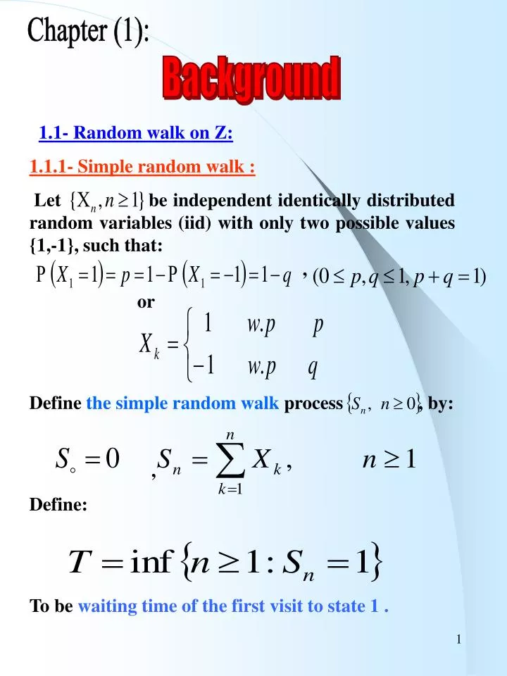
1.1- Random walk on Z: 1.1.1- Simple random walk : Let be independent identically distributed random variables (iid) with only two possible values {1,-1}, such that: , or

E N D
1.1- Random walk on Z: 1.1.1- Simple random walk : Let be independent identically distributed random variables (iid) with only two possible values {1,-1}, such that: , or Define the simple random walk process , by: , Define: To be waiting time of the first visit to state 1 . Chapter (1): Background
A state (i) is called recurrent if the chain returns to (i) with probability 1 in a finite number of steps, other wise the state is transient. If we define the waiting time variables as , then state i is recurrent if . That is the returns to the state (i) are sure events , and the state (i) is transient if: In this case there is positive probability of never returning to state (i), and the state (i) is a positive recurrent if . Hence if then the state (i) is a null recurrent . 1.2-Transience and recurrence:
1.2.1-Definition: We say that i leads to (j) and write if for some We say i communicates with j and write if both and . 1.2.2-Definition: A Markov chain with state space S is said to be irreducible if , 1.2.3-Theorem: If x is recurrent and then y is recurrent.
1.2.4-Lemma: If the Markov chain is irreducible, and one of the states is recurrent then all the states are recurrent . 1.2.5-Lemma: 1) If and , then . 2) If and , then . 1.2.6-Theorem : The simple random walk on is recurrent iff
5.12- Now we will prove theorem (1.2.6) in chapter (1): We define the state or position of random walk at time zero as , and the position at time n as , then by strong law of large number Because: are independent identically distributed and from the definition ,then . Hence And This means that and consequence of that we have The state 0 is transient if the number of visit to zero is finite almost surly, which mean that with probability 1 the number of visit is finite .
Hence zero is transient state. Now if p=q=1/2, we claim recurrence. It is enough to show that 0 is recurrent (from theorem 1.2.4), then the state 0 is recurrent iff Define Where
Now using sterling formula Hence However and 0 is recurrent, and consequently the simple random walk on Z is recurrent . Now we will show that symmetric simple random walk is null recurrent, which means that Where
The probability generating function is defined as: Then Also Hence And
5.12.1-Another proof: We proved that simple random walk on Z is recurrent if . We have: Then: Put: Hence: and Hence zero is a null recurrent, and the simple symmetric random walk on Z is null recurrent.
1.3- Borle-Cantelli lemma : If is an infinite sequence of events such that: 1. 2. , provided that are independent events.
The 1st Example: It is well known that ifare independent random variables , then , but this may fail in the case of infinite product ,To show this we can introduce this counter example . Chapter (2): Some Counter Examples Of Probability
* Consider to be independent random variables such that: That is we have infinite sequence of independent identically distributed random variables, then: We define anew sequence as follows: then Now define the waiting time that means the first time the sequence equal to zero. Then :
On the other hand hence: T is finite almost surly.
2.2.1-Definition i. X is finite random variable iff ii. X is bounded iff Now we introduce the notion of lebesgue measure, and Borel -field 2.2- Introduction to the second example
· The -field is a collection of sub-sets of such that 1. 2. 3. The elements of are called measurable sets or events. * The intersection of all -fields that contain all open intervals is called Borel -fieldand denoted by. It is known thata lebesgue measureon (Borel -field) is the only measure that assigns for every interval (a,b] a measure , and . 2.2.3- Theorem (1) : Provided that EX and EY are finite. 2.2.2-Definitions:
2.2.4- Theorem (2): If is finite then: Note : If are independent identically distributed random variables, and N is positive integer valued random variable independent of then: Proof: and Hence
2.2.5- Theorem (3) : (Monotone convergence theorem) If , and Then 2.2.6- Theorem (4) : If random variables, then Proof: We define a new sequence then: now
·But is this theorem true if ? The following example shows that this theorem may fail if all . Define are independent identically distributed random variables, such that: and define : and 2.3- The 2nd Example:
Because we have symmetric simple random walk, then recurrence implies that and then: Define also: then: On the other hand :
The sigma-field generated by a random variable X is: where is the Borel . the event does occur or does not depending only on , which means that . Hence are independent random variables. then and Hence from (2) & (3) we conclude that: .
* The following example shows that the formula (1) may not be true. A common error is repeated in some books, about linear correlation which is But this relation must be written as: * Consider a random variable . We define the triple where and and P=Lesbgue measure on . is the Borel -field restricted on (0,1) . 2.4- The 3rd Example:
Suppose for the contrary that Now define From (1) & (2) we get a = 0 , y = b This Contradiction because the assumption is not true.
3.1- The 4th Example: It is already known that if the moment generating function do exist ,then all the moment do exist ,but it could happen that all the moments do exist but the moment generating function does not exist, the following counterexample explains this We know if the moment generating function is defined , then Let Chapter (3): Some Counterexamples Of Statistics
And define , that is Y follows the lognormal distribution. Hence all the moment of y do exist, whereas the moment generating function of Y does not exist, as we show now . Then the moment generating function does not exist.
3.2- The 5th Example: The sequence of moments does not determine uniquely the distribution, the following example show this: We have the following two distributions with identical sequence of moments
Now: Obviously . Also
3.2.1-Theorem: It is known from the literature that the sequence of moments of a random variable uniquely determines the distribution if it satisfies one of the following equivalent conditions:
Y X 0 1 ; 0 1 3.3- The 6th Example: The joint distribution of random variables determines uniquely the marginal distributions, but the converse is not necessarily true . This is a joint probability function
The marginal distribution of X is: X 0 1 The marginal distribution of Y is: Y 0 1 These two marginal functions are corresponding to the joint function fir any Conclusion: The marginal distributions don’t determine the joint distribution.
A matrix is said to be positive definite if it satisfies one of the following equivalent conditions: i. ii. All the eignvalues are positive. iii. The determinants of all left upper sub-matrices are positive. 3.4- The 7th Example: The “positive correlated” is not transitive property. 3.4.1-Theorem:
We can make sure that is variance-covariance matrix of a random variable . then 3.4.2-Theorem: Any positive definite matrix could be variance-covariance matrix of some random vector. · Now Consider the matrix Then X and Y are positively correlated, and Y and Z as well, but X and Z are negatively correlated
We say that converges weakly to X if: At all continuity points of F. This is denoted by or 3.4.3-Definition: The following example shows that a sequence of continuous random variable does not necessary converge weakly to a continuous random variable.
Obviously, is the cumulative distribution function of a continuous random variable . Whereas, F is the cumulative distribution function of a discrete random variable X. Never the less, . 3.5- The 8th Example: Let Then X is a degenerate random variable with cumulative distribution function Consider a sequence of cumulative density functions such that: Then
Let X be a random variable such that The median is any x such that If F is continuous random variable, then the median is unique . 3.6- THE MEDIAN 3.6.1-Definition:
The cumulative density function of X thus the median is any Which means that a=0, and b=1. That is, the median is not unique. This is a disadvantage of the median as a measure of location as the mean . 3.6.2-Example: Consider a random variable X, such that X -1 0 1 2 P(X)
Assume that Y is an independent copy of X, so we can find Med(X) and Med(Y) as follows 3.7- The 9th Example: The median does not satisfy the relation Mod(X+Y) = Mod(X) + Mod(Y) If Then : Let then
this implies that Med(X) =Med(Y)=log2 now to calculated Med (Z) suppose for contrary that Med(X+Y) = Med(X) + Med(Y) This means that Med(Z) = 2 log 2 With probability density function
. If the median of Z were 2log 2, then However, Hence
A random variable X has the following distribution X 0 1 2 P(X) The mode is not unique, it is 0 and 1 3.8-The Mod The mod is the value of X that makes the density function is maximum. 3.8.1-Example:
X 0 1 P(X) Z 0 1 2 P(Z) The 10th Example: We show in this example that the mode is not a linear operator. This is a disadvantage of the mode. i. For discrete random variable Suppose that X&Y follow the distribution above and they are independent. Let Z=X+Y
Let and Y is an independent copy of X, Since f (0)=1 is the maximum value of f(x), hence Now Z = X + Y, then , the probability density function of Z i. For continuous random variable and from (1) & (2) we conclude that the Mode is not linear operator.
We defined a simple random walk in chapter (1), and we know that the following Markov Chain is recurrent iff This walk is called simple symmetric random walk (SSRW). Chapter (4): SIMPLE RANDOM WALK ON Z 4.1) Simple symmetric random walk:
4.1.1) Theorem: Simple symmetric random walk (SSRW) on Z is irreducible Proof : Consider a state i and a state j such that: ( Transitive property) . By the same way Hence simple symmetric random walk (SSRW) on Z is irreducible.
4.2) Martingale A sequence of random variables is Martingale if: and sub-martingale if and a super-martingale if :
4.2.1) Example: Consider independent random variables , such that We claim that is a martingale, for
4.2.2) Example: Consider independent random variables Define a sequence . We show that is a martingale. Proof
Consider a family tree where , and let the number of children at generation , and let the number of children of the generation then: individual of the and is a doubly indexed family . ,then We assume that Variables, for every n and k and for fixed n they are independent identically distributed random variables. 4.3-Family tree ’s independent random
, we Show that Consider , then is a martingale. Proof are We use the fact that: If Independent identically distributed random variables and Integer-valued random variable and independent of then: 4.3.1) Example:
Since are independent of Then: And æ ö Z n å ç Á E d ç nk n æ ö Z è ø E = ç k 1 Á = n ç n EZ EZ Ed è ø + n 1 n n ( ) Á Z E d = n n 1 n EZ Ed n n Z Ed = n n 1 EZ Ed n n Z = = n W n EZ n are independent random variables, and for fixed n they are independent identically distributed. Also
4.4 - The 11th Example: Almost sure limit of the martingales. (Not every martingale has an almost sure limit). In a symmetric simple random walk on Z, we have , then is a martingale since and does not exist, because this symmetric simple random walk (SSRW), is recurrent this means that it keeps oscillating between all the integers.