Download
1 / 22
220 likes | 333 Views
Esci 203, Earth Structure and Deformation Introduction to the global positioning system (GPS). John Townend EQC Fellow in Seismic Studies john.townend@vuw.ac.nz. Recent events.

E N D
Esci 203, Earth Structure and DeformationIntroduction to the global positioning system (GPS) John Townend EQC Fellow in Seismic Studies john.townend@vuw.ac.nz
Recent events Preliminary GPS displacement data (version 0.1) provided by the ARIA team at JPL and Caltech. All Original GEONET RINEX data provided to Caltech by the Geospatial Information Authority (GSI) of Japan.
Overview • What is GPS • A space-based Global Positioning System • How does it work? • Trilateration using very accurate timing measurements • What are some of its limitations? • How can earth scientists use it? • General positioning, deformation monitoring…
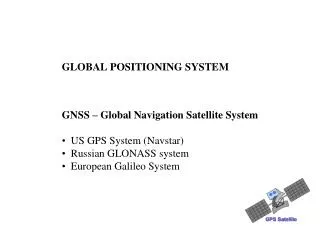
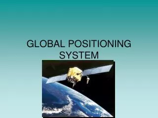
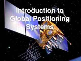
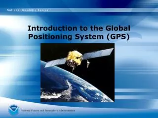
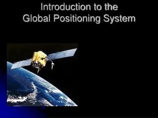
What is GPS? • Space segment, Navstar • 24 satellites orbiting at an altitude of ~20,000 km • Control segment • 5 ground stations • User segment • Users with GPS receivers Global Positioning System
Campaign and permanent GPS Continuous (permanent) GPS station Gisborne, New Zealand Campaign (temporary) GPS station Pu`u O`o, Kilauea, Hawai`i • Figures courtesy of Peter Cervelli, HVO, and Land Information New Zealand
The satellite signal • Each satellite transmits low-power (20–50 W) signals on various frequencies • Civilian receivers listen at 1575.42 MHz • The receiver determines the signal travel time from the satellite • With four or more satellites, the receiver can determine its latitude, longitude, altitude, and internal clock error
Pseudo-random codes • The signal emitted by each satellite is unique and extremely complex (“pseudo-random”) • The receiver generates the same signal, and compares it with what it receives from the satellite to determine the travel time Receiver signal t Satellite signal
Extra steps • What is the time? • Each satellite carries an atomic clock but the receiver’s internal clock is much less accurate • So, the receiver uses an extra satellite signal to estimate the difference in time between it’s onboard clock and the standardised satellite time • And where are the satellites exactly? • The control stations measure each satellite’s ephemeris very precisely; this data is broadcast to the satellites and included in the GPS signal
Sat1 Sat2 Sat3 Sat4 Trilateration • The receiver determines the distance (“pseudo-range”) to 4+ satellites, and calculates its position; it’s like locating an earthquake in reverse! distance = travel time speed of light
Sources of error • Ionospheric/tropospheric delays • Multi-pathing • Receiver clock errors • Ephemeris errors • Constellation geometry and weather • Intentional signal degradation: • “selective availability”, which limited accuracy to ~6–12 m but has now been switched off
Selective availability Figure courtesy of Peter Cervelli, HVO
Geometric dilution of precision High GDOP; low confidence Low GDOP; high confidence
Differential GPS (“dGPS”) • Reference stations broadcast corrections to the satellites’ signals; typical dGPS accuracy is ~1–5 m Satellite GPS signal GPS signal dGPS correction signal Mobile receiver Reference station
vE vN v Geodetic velocities We commonly make use of the east and north components of velocity, vE and vN The overall velocity vector v has a magnitude (length), v2 = vE2 + vN2, and an azimuth = atan (vE/vN)
Measuring velocities The velocity in each direction (east, north, up) is just the gradient of the position time series
Measuring velocities n t The velocity in each direction (east, north, up) is just the gradient of the position time series e.g. vN = n/t
Relative motion (1) vair-ground vplane-ground = vplane-air + vair-ground vplane-air
Relative motion (2) vB-ref vA-ref = vA-B + vB-ref vA-B meaning that vA-B = vA-ref – vB-ref = vA-ref + (– vB-ref)
Relative motion (3) Site B vB –vB vB vA-B vA vA Site A
Summary • Points to revise • How GPS basically works • Key factors affecting position estimates • Measuring site velocities from GPS data and relative velocities between sites • Extra material online • http://ww2.trimble.com/gps_tutorial
Reading material • Van der Pluijm and Marshak • Section 14.9 • Fowler (2005) • Sections 2.1 and 2.2 • Mussett and Khan • Section 20.5 • If you need to brush up on vectors, try “Mathematics : a simple tool for geologists”, by Waltham; this is in the library