Download
1 / 24
240 likes | 378 Views
Approximate Inference for Complex Stochastic Processes: Parametric & Nonparametric Approaches. Brenda Ng & John Bevilacqua 16.412J/6.834J Intelligent Embedded Systems 10/24/2001. Overview. Problem statement

E N D
Approximate Inference for Complex Stochastic Processes: Parametric & Nonparametric Approaches Brenda Ng & John Bevilacqua 16.412J/6.834J Intelligent Embedded Systems 10/24/2001
Overview Problem statement Given a complex system with many state variables that evolve over time, how do we monitor and reason about its state? • Robot localization and map building • Network for monitoring freeway traffic Approach • Representation: Model problem as a Dynamic Bayesian Network • Inference: Approximate inference techniques • Exact inference on approximate model Parametrized approach: Boyen-Koller Projection • Approximate inference on exact model Nonparametrized approach: Particle Sampling Contribution Reduce complexity of problem via approximate methods, rendering the problem of monitoring complex dynamic system tractable.
What is a Bayesian Network? A Bayesian network, or a belief network, is a graph in which the following holds: • A set of random variables makes up nodes of the network. • A set of directed links connects pairs of nodes to denote causality relations between variables. • Each node has a conditional probability distribution that quantifies the effects that the parents have on the node. • The graph is directed and acyclic. Courtesy of Russell & Norvig
Why Bayesian Networks? Season x1 • Bayesian networks achieve compactness by factoring the joint distribution into local, conditional distributions for each variable given its parents. x2 x3 Rain Sprinkler x4 Wet Slippery x5 • Bayesian networks lend easily to evidential reasoning.
Dynamic Bayesian Networks Dynamic Bayesian networks capture the process of variables changing over time by representing multiple copies of state variables, one for each time step. • A set of variables X denotes the world state at time t and a set of sensor variables E denotes the observations available at time t. • Keeping track of the world means computing the current probability distribution over world states given all past observations, P(Xt|E1,…,Et). • Observation model P(Et|Xt) and transition model P(Xt+1|Xt) Courtesy of Koller & Lerner
Why Approximate Inference? The variables in a DBN can become correlated very quickly as the network is unrolled. Consequently, no decomposition of the belief state is possible and exact probabilistic reasoning methods is infeasible.
Monitoring Task I Belief state at time t-1: {t-1)[si] State evolution model: T Prior distribution: Observation at time t Observation model: O Posterior distribution: Belief state at time t: {t )[si]
Monitoring Task II Belief state at time t: {t)[si] State evolution model: T (t•) Prior distribution: Observation at time t+1 Observation model: O Posterior distribution: Belief state at time t+1: {t+1 )[si]
Boyen-Koller Projection Algorithm • Decide on some computationally tractable representation for an approximate belief state, e.g. one that decomposes into independent factors. • Propagate the approximate belief state at time t through the transition model and condition it on our evidence at time t+1. • In general, the resulting state for time t+1 will not fall into the class which we have chosen to maintain. • Continue to approximate the belief state using one that does and continue. Assumptions • T is ergodicfor error to be bounded. • The approximate belief state must bedecomposable. Approximation Error • Gradual accumulation of approximation errors • Spontaneous amplification of error due to instability
~ Approximate belief state at time t: {t)[si] Prior distribution: ~ ^ ^ Posterior distribution: ^ ^ ^ Belief state approximation: Project (t+1•) ~ Approximate belief state at time t+1: {t+1)[si] Monitoring Task (Revisited) State evolution model: T (t•) Observation at time t+1 Observation model: O
Approximation Error Approximation error results from two sources: • old error “inherited” from the previous approximation (t) • new error derived from approximating (t+1) using (t+1) Suppose that each approximation introduces an error of , increasing the distance between the exact belief state and our approximation to it. How is the error going to be bounded? ~ ~ ^
Idea of Contraction • To insure that the error is bounded means T and O must reduce the distance between the two belief states by a constant factor. • Distance Measure • If j and y are two distributions over the same space W, the relative entropy of j and y is: s(t ) error ~ s(t ) Point of convergence
Contraction Results These contraction results show that the approximate belief state and the true belief state are driven closer to each other at each propagation of the stochastic dynamics. Thus, the BK approximation method never introduces unbounded error! BK is a stable approximation method!
Rao-Blackwellised Particle Filters • Sampling-based inference/learning algorithms for Dynamic Bayesian Networks • Exploit the structure of a DBN by sampling some of the variables and marginalizing out the rest in order to increase the efficiency of particle filtering • Lead to more accurate estimates than standard Particle Filters
bt=P(st| ht) P(st|ht) P(st+1|at,ht) bt=P(st+1| ht+1) Ht+1= zt+1,at,ht Particle Filtering • Resample Particles 2) Propagate according to action a1 3) Reweight according to observation zt+1
Rao-Blackwellization Conditions for using RBPFs • The system contains discrete states and discrete observations. • The system contains variables which can be integrated out analytically. Algorithm • Decompose dynamic network via factorization. • Identify variables whose value can be discerned by observation of the system and other variables. • Perform particle filtering on these variables and compute relevant sufficient statistics.
Example of Rao-Blackwellization • Have a system with variables time, position, velocity • Realize that, given the current and previous position and time, velocity can be determined • Remove velocity from system model and perform particle filtering on position • Based on sampled value for position, calculate the distribution for the velocity variable
Application: Robot Localization I Robot Localization & Map Building Scenario A robot can move on a discrete, 1D grid. Objective To learn a map of the environment, represented as a matrix that stores the color of each grid cell. Sources of Stochasticity • Imperfect sensors • Mechanical faults (motor failure & wheel slippage) The robot needs to know where it is to learn the map, but needs to know the map to figure out where it is.
Application: Robot Localization II A. Exact inference B. RBPF with 50 samples C. Fully-factorized BK Summary of results • RBPF is able to provide near the same accuracy of estimation as exact inference. • BK gets confused because it ignores correlations between the map cells.
Application: BAT Network I Analysis procedures • Process is monitored using the BK/sampling method with some fixed decomposition or some fixed number of particles. • Performance is compared with the result derived from exact inference. BAT network used for monitoring freeway traffic
BAT Results: BK • The errors obtained in practice is significantly lower than that predicted by the theoretical analysis. • This algorithm works optimally when clusters are chosen to correspond to structure of weekly correlated subprocesses. • Accuracy can be further improved by using conditionally independent approximations. • Evidence boosts contraction and significantly reduce the overall error of our approximation. (Good for likely evidence, bad for unlikely evidence). • By exploiting structure of a process, this approach can achieve orders of magnitude faster inference with only a small degradation inaccuracy.
BAT Results: Sampling • Error drops sharply initially and then the improvements become smaller and smaller. • The average KL-error changes dramatically over the sequence. The spikes correspond to unlikely evidence, in which case the samples become less reliable. This suggests that a more adaptive sampling scheme may be advantageous. • Particle filtering gives a very good estimate of the true distribution over the variable.
BK vs. RBPF • Boyen-Koller projection • Applicable for inference on networks with structure that lends easily to decomposition • Requires transition model to be ergodic • Rao-Blackwellized particle filters • Applicable for inference on networks with redundant information • Applicable for difficult distributions
Contributions • Introduced Dynamic Bayesian Networks and explained their role in inference of complex stochastic processes • Examined two different approaches to analyzing DBNs • Exact Computation on an approximate model: BK • Approximate Computation on an exact model: RBPF • Compared performance and applicability of these two approaches