Download
1 / 26
300 likes | 500 Views
JPEG Compression. What is JPEG? "Joint Photographic Expert Group". Voted as international standard in 1992. Works with color and grayscale images, e.g., satellite, medical, ... Motivation

E N D
JPEG Compression • What is JPEG? • "Joint Photographic Expert Group". Voted as international standard in 1992. • Works with color and grayscale images, e.g., satellite, medical, ... • Motivation • The compression ratio of lossless methods (e.g., Huffman, Arithmetic, LZW) is not high enough for image and video compression, especially when the distribution of pixel values is relatively flat.
JPEG Compression 1-D Discrete Cosine Transform • A cosine transform is required to compute on a set of N even functioned periodic data points with a sampling interval Ts. The data is made even functioned by folding about the vertical axis. This gives an even periodic function but 2N-1 data points. • By offsetting the sampling point by Ts/2 and then folding the points about the vertical axis an even periodic function is obtained with 2N points
JPEG Compression 1-D Discrete Cosine Transform: Example • Applying a discrete cosine transform of length 2N to the data xn where n = -N to (N-1).
JPEG Compression 1-D Discrete Cosine Transform: Example • The forward transform matrix is symmetrical about the A axis. Folding about A axis allows the x(k) coefficients to be computed from the positive x(n) samples (0 to N-1) and forward DCT transform becomes: • The reverse transform matrix is symmetrical about the B axis. Folding about B axis allows the x(n) coefficients to be computed from the positive x(k) samples (0 to N-1) and reverse DCT transform becomes: where C0 = 1 when k 0 and C0 = 1/2 when k = 0 • Combining the folds and sharing the scaling factor between the forward and reverse transforms allows the basis matrix to be the same and yields the following forward and reverse transforms: where C0 = 1 when k 0 and C0 = 1/2 when k = 0
JPEG CompressionDiscrete Cosine Transform (DCT) • From spatial domain to frequency domain:
JPEG Compression Properties • DCT is like FFT, but can approximate linear signals well with few coefficients
JPEG CompressionTwo 1-D DCTs • Factoring allows 2-D DCT to be computed as a series of 1D DCTs • Most software implementations use fixed point arithmetic. Some fast implementations approximate coefficients so all multiplies are shifts and adds
JPEG CompressionQuantization • F'[u, v] = round ( F[u, v] / q[u, v] ). • Reduce number of bits per sample • Example: 101101 = 45 (6 bits). q[u, v] = 4 --> Truncate to 4 bits: 1011 = 11. • Quantization error is the main source of the Lossy Compression. • Uniform Quantization • Each F[u,v] is divided by the same constant N.
JPEG CompressionNon-uniform Quantization • Eye is most sensitive to low frequencies (upper left corner), less sensitive to high frequencies (lower right corner) • Quantization tables used to generate non-uniform quantisation • The Luminance Quantization Table q(u, v) The Chrominance Quantization Table q(u, v) • The numbers in the above quantization tables can be scaled up (or down) to adjust the so called quality factor. • Custom quantization tables can also be put in image/scan header.
JPEG CompressionZig-Zag Scan • Groups low frequency coefficients in top of vector • Maps 8 x 8 to a 1 x 64 vector
JPEG Compression: DC & AC Component Coding • Differential Pulse Code Modulation (DPCM) on DC component • DC component is large and varied, but often close to previous value • Encode the difference from previous 8 x 8 blocks -- DPCM • Run Length Encode (RLE) on AC components • 1 x 64 vector has lots of zeros in it • Keeps skip and value, where skip is the number of zeros and value is the next non-zero component. • Send (0,0) as end-of-block sentinel value
JPEG CompressionEntropy Coding • Categorize DC values into SIZE (number of bits needed to represent) and actual bits. • Example: if DC value is 4, 3 bits are needed. • Send off SIZE as Huffman symbol, followed by actual 3 bits. • For AC components two symbols are used: Symbol_1: (skip, SIZE), Symbol_2: actual bits. Symbol_1 (skip, SIZE) is encoded using the Huffman coding, Symbol_2 is not encoded. • Huffman Tables can be custom (sent in header) or default.
JPEG CompressionFour JPEG Modes • Sequential Mode • Lossless Mode • Progressive Mode • Hierarchical Mode
JPEG CompressionSequential Mode • Each image component is encoded in a single left-to-right, top-to-bottom scan. • Baseline Sequential Mode, the one that we described above, is a simple case of the Sequential mode: • It supports only 8-bit images (not 12-bit images) • It uses only Huffman coding (not Arithmetic coding)
JPEG CompressionSequential Mode • Each image component is encoded in a single left-to-right, top-to-bottom scan.
JPEG CompressionLossless Mode • A special case of the JPEG where indeed there is no loss. • It does not use DCT-based method! Instead, it uses a predictive method.
JPEG CompressionLossless Mode (cont) • A predictor combines the values of up to three neighboring pixels (not blocks as in the Sequential mode) as the predicted value for the current pixel, indicated by "X" in the figure below. The encoder then compares this prediction with the actual pixel value at the position "X", and encodes the difference losslessly.
JPEG CompressionLossless Mode (cont) • It can use any one of the following seven predictors • Since it uses only previously encoded neighbors, the very first pixel I(0, 0) will have to use itself. Other pixels at the first row always use P1, at the first column always use P2. • Effect of Predictor (test result with 20 images): (Predictor Selection Value)
JPEG CompressionProgressive Mode • Goal: display low quality image and successively improve. • Two ways to successively improve image: • Spectral selection: Send DC component and first few AC coefficients first, then gradually some more ACs. • Successive approximation: send DCT coefficients MSB (most significant bit) to LSB (least significant bit). (Effectively, it is sending quantized DCT coefficients frist, and then the difference between the quantized and the non-quantized coefficients with finer quantization stepsize.)
JPEG CompressionHierarchical Mode • Down-sample by factors of 2 in each dimension, e.g., reduce 640 x 480 to 320 x 240 • Code smaller image using another JPEG mode (Progressive, Sequential, or Lossless). • Decode and up-sample encoded image • Encode difference between the up-sampled and the original using Progressive, Sequential, or Lossless.
JPEG CompressionHierarchical Mode (cont) • Can be repeated multiple times. • Good for viewing high resolution image on low resolution display.
JPEG Compression JPEG 2000 • JPEG 2000 is the upcoming standard for Still Pictures (due Year 2000). • Among many things it will address: • Low bit-rate compression performance, • Lossless and lossy compression in a single codestream, • Transmission in noisy environment where bit-error is high, • Application to both gray/color images and bi-level (text) imagery, natural imagery and computer generated imagery, • Interface with MPEG-4, • Content-based description.