Download
1 / 21
210 likes | 310 Views
The Normal Curve. Probability Distribution. Imagine that you rolled a pair of dice. What is the probability of 5-1 ? To answer such questions, we need to compute the whole population for possible results of rolling two dices.

E N D
Probability Distribution • Imagine that you rolled a pair of dice. What is the probability of 5-1? • To answer such questions, we need to compute the whole population for possible results of rolling two dices. • A standard dice has six faces. The probability of a number on a dice is 1/6.
Probability Distribution • We have two unrelated populations. That is, the results of the dices are not dependent. • So, the probability of 5-1 is equal to 1/6 * 1/6 = 1/36. That means, in the perfect universe of math, if we roll two dice for 36 times, than one of the results will be 5-1. • We can see that in the table below
Probability Distribution So, the probability of 5 – 1 is 1/36. But remember, it is the probability of the event that the first dice (and only the first one) will be 5 and the second one will be 1
Probability Distribution • What if we would like to find the probability of the number 6 in that table? • That is the events when the sum of the two dices will be six. • Which combinations of two dices produce the score 6? • Let’s see in the same table
Probability Distribution • So, the probability of the score 6 is 5/36. • That is, in the perfect conditions 5 of 36 trails will result in the score 6.
Probability Distribution • Now, to see the distributions of the possible score, let’s compute the possibilities of each scores ranging between 2 – 12. Let’s relook at the table
Probability Distribution • Now, let’s look at the shape of distribution.
Basic Characteristics of Normal Curve • There are different kinds of normal curves. • Their means and standard deviations differ from each other. But, the matter of concern is their shape. • Three possible conditions for normal curves are
Basic Characteristics of Normal Curve • As you can see, the main similarity of the different normal curves is their symmetrical shape. • That is, the left half of the normal distribution is a mirror image of the right half • They are unimodal distributions, with the mode at the center • Mode, median and mean have the same value. • Their tails never touches to the x axis. So, we describe the area under the curve as proportion. That is, the total area under the curve is equal to 1
Basic Characteristics of Normal Curve • The equation of normal curve is:
Basic Characteristics of Normal Curve • As you can see, the value of Y is determined by N, sd, mean. So, different distributions with different N, sd and mean have different normal distributions. Basically, • N= the area under the curve • Mean= location of the center of the curve • SD= rapidity with which the curve approaches to x axis.
Basic Characteristics of Normal Curve • As you can remember, to standardize different distributions, we use z scores. The mean and sd of z scores is 0 and 1, respectively. So, if we reorganize the formula for z, it becomes
Basic Characteristics of Normal Curve • As you can see, last formula indicates that z score determines the area in the normal curve. • So, using the standardized z scores, we can compute areas in the normal curve • In book, you can see these areas in Table A, pp. 552
Area Under the Normal Curve • In Table A, • z scores, • the area between z scores and mean, • and the area above z scores are presented. • Note 1: the areas are bigger when z score is close to zero (the mean) • Note 2: the sum of the two areas (the area between z scores and mean, AND the area above z scores) is .50. Because, this area represents the half of the distribution • Note 3: All z scores in the distribution are positive, since the possitive area are the mirror image of negative area
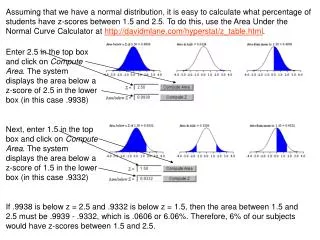
Area Under the Normal Curve • Using this table, we can calculate • The area above a certain score • How many students (what proportion of scores) got (was) higher than 70 in the final prep. exam • The area under a certain score • How many students got lower than 35 points in the final prep. exam • The area two known scores • How many students got a score btw. 35 and 70 points in the final prep. exam
Area Under the Normal Curve • The area above a certain score • The mean of the prep. Final exm = 60 • The SD is 10 • 2500 students took the final exam