Quantifying Uncertainty in Belowground Carbon Turnover

1. Quantifying Uncertainty in Belowground Carbon Turnover Ruth D. Yanai State University of New York College of Environmental Science and Forestry Syracuse NY 13210, USA

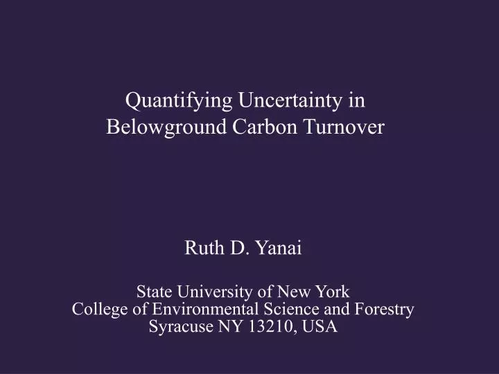
2. QUANTIFYING UNCERTAINTY IN ECOSYSTEM STUDIES Quantifying uncertainty in ecosystem budgets Precipitation (evaluating monitoring intensity) Streamflow (filling gaps with minimal uncertainty) Forest biomass (identifying the greatest sources of uncertainty) Soil stores, belowground carbon turnover (detectable differences)

3. UNCERTAINTY Natural Variability Knowledge Uncertainty Spatial Variability Measurement Error Temporal Variability Model Error Types of uncertainty commonly encountered in ecosystem studies Adapted from Harmon et al. (2007)

4. How can we assign confidence in ecosystem nutrient fluxes? Bormann et al. (1977) Science

5. The N budget for Hubbard Brook published in 1977 was “missing” 14.2 kg/ha/yr Bormann et al. (1977) Science

6. The N budget for Hubbard Brook published in 1977 was “missing” 14.2 kg/ha/yr 14.2 ± ?? kg/ha/yr • Net N gas exchange = sinks – sources = • precipitation N input • + hydrologic export • + N accretion in living biomass • + N accretion in the forest floor • ± gain or loss in soil N stores

7. The N budget for Hubbard Brook published in 1977 was “missing” 14.2 kg/ha/yr 14.2 ± ?? kg/ha/yr • Net N gas exchange = sinks – sources = • precipitation N input • + hydrologic export • + N accretion in living biomass • + N accretion in the forest floor • ± gain or loss in soil N stores

8. Measurement Uncertainty Sampling Uncertainty Spatial and Temporal Variability Across catchments: 3% Across years: 14% Undercatch: 3.5% Model Uncertainty Error within models Error between models Volume = f(elevation, aspect): 3.4 mm Model selection: <1%

10. We tested the effect of sampling intensity by sequentially omitting individual precipitation gauges. Estimates of annual precipitation volume varied little until five or more of the eleven precipitation gauges were ignored.

11. The N budget for Hubbard Brook published in 1977 was “missing” 14.2 kg/ha/yr 14.2 ± ?? kg/ha/yr • Net N gas exchange = sinks – sources = • precipitation N input (± 1.3) • + hydrologic export • + N accretion in living biomass • + N accretion in the forest floor • ± gain or loss in soil N stores

12. The N budget for Hubbard Brook published in 1977 was “missing” 14.2 kg/ha/yr 14.2 ± ?? kg/ha/yr • Net N gas exchange = sinks – sources = • precipitation N input (± 1.3) • + hydrologic export • + N accretion in living biomass • + N accretion in the forest floor • ± gain or loss in soil N stores

14. Don Buso HBES

15. Gaps in the discharge record are filled by comparison to other streams at the site, using linear regression.

16. Cross-validation: Create fake gaps and compare observed and predicted discharge Gaps of 1-3 days: <0.5% Gaps of 1-2 weeks: ~1% 2-3 months: 7-8%

17. The N budget for Hubbard Brook published in 1977 was “missing” 14.2 kg/ha/yr 14.2 ± ?? kg/ha/yr • Net N gas exchange = sinks – sources = • precipitation N input (± 1.3) • + hydrologic export (± 0.5) • + N accretion in living biomass • + N accretion in the forest floor • ± gain or loss in soil N stores

18. The N budget for Hubbard Brook published in 1977 was “missing” 14.2 kg/ha/yr 14.2 ± ?? kg/ha/yr • Net N gas exchange = sinks – sources = • precipitation N input (± 1.3) • + hydrologic export (± 0.5) • + N accretion in living biomass • + N accretion in the forest floor • ± gain or loss in soil N stores

19. Monte Carlo Simulation Monte Carlo simulations use random sampling of the distribution of the inputs to a calculation. After many iterations, the distribution of the output is analyzed. Yanai, Battles, Richardson, Rastetter, Wood, and Blodgett (2010) Ecosystems

20. A Monte-Carlo approach could be implemented using specialized software or almost any programming language. Here we used a spreadsheet model.

21. Lookup Lookup Lookup Height Parameters ***IMPORTANT*** Random selection of parameter values happens HERE, not separately for each tree • Height = 10^(a + b*log(Diameter) + log(E))

22. If the errors were sampled individually for each tree, they would average out to zero by the time you added up a few thousand trees

23. Biomass Parameters Lookup Lookup Lookup • Biomass = 10^(a + b*log(PV) + log(E)) • PV = 1/2 r2 * Height

24. Biomass Parameters Lookup Lookup Lookup • Biomass = 10^(a + b*log(PV) + log(E)) • PV = 1/2 r2 * Height

25. Biomass Parameters Lookup Lookup Lookup • Biomass = 10^(a + b*log(PV) + log(E)) • PV = 1/2 r2 * Height

26. Concentration Parameters Lookup Lookup • Concentration = constant + error

27. COPY THIS ROW-->

28. Paste Values button After enough interations, analyze your results

29. Biomass of thirteen stands of different ages C1 C2 C3 C4 C5 C6 HB-Mid JB-Mid C7 C8 C9 HB- Old JB-Old Young Mid-Age Old

30. Coefficient of variation (standard deviation / mean) of error in allometric equations 3% 2% 4% 4% 5% 4% 4% 3% 3% 3% 3% 7% 3% C1 C2 C3 C4 C5 C6 HB-Mid JB-Mid C7 C8 C9 HB- Old JB-Old Young Mid-Age Old

31. CV across plots within stands (spatial variation) Is greater than the uncertainty in the equations 16% 10% 19% 3% 11% 3% 2% 4% 4% 5% 12% 12% 18% 13% 14% 4% 4% 3% 3% 3% 6% 15% 11% 3% 7% 3% C1 C2 C3 C4 C5 C6 HB-Mid JB-Mid C7 C8 C9 HB- Old JB-Old Young Mid-Age Old

33. Better than the sensitivity estimates that vary everything by the same amount--they don’t all vary by the same amount! “What is the greatest source of uncertainty in my answer?”

34. “What is the greatest source of uncertainty to my answer?” Better than the uncertainty in the parameter estimates--we can tolerate a large uncertainty in an unimportant parameter.

36. The N budget for Hubbard Brook published in 1977 was “missing” 14.2 kg/ha/yr 14.2 ± ?? kg/ha/yr • Net N gas exchange = sinks – sources = • precipitation N input (± 1.3) • + hydrologic export (± 0.5) • + N accretion in living biomass (± 1) • + N accretion in the forest floor • ± gain or loss in soil N stores

37. The N budget for Hubbard Brook published in 1977 was “missing” 14.2 kg/ha/yr 14.2 ± ?? kg/ha/yr • Net N gas exchange = sinks – sources = • precipitation N input (± 1.3) • + hydrologic export (± 0.5) • + N accretion in living biomass (± 1) • + N accretion in the forest floor • ± gain or loss in soil N stores

38. Oi Oe Oa E Bh Bs Forest Floor Mineral Soil

39. 10 points are sampled along each of 5 transects in 13 stands.

40. Excavation of a forest floor block (10 x 10 cm)

41. Pin block is trimmed to size. Horizons are easy to see.

42. Horizon depths are measured on four faces Oe, Oi, Oa and A (if present) horizons are bagged separately In the lab, samples are dried, sieved, and a subsample oven-dried for mass and chemical analysis.

43. Nitrogen in the Forest Floor Hubbard Brook Experimental Forest

44. Nitrogen in the Forest Floor Hubbard Brook Experimental Forest The change is insignificant (P = 0.84). The uncertainty in the slope is ± 22 kg/ha/yr.

45. The N budget for Hubbard Brook published in 1977 was “missing” 14.2 kg/ha/yr 14.2 ± ?? kg/ha/yr • Net N gas exchange = sinks – sources = • precipitation N input (± 1.3) • + hydrologic export (± 0.5) • + N accretion in living biomass (± 1) • + N accretion in the forest floor (± 22) • ± gain or loss in soil N stores

46. Studies of soil change over time often fail to detect a difference. We should always report how large a difference is detectable. Yanai et al. (2003) SSSAJ

47. Power analysis can be used to determine the difference detectable with known confidence

48. Sampling the same experimental units over time permits detection of smaller changes

49. In this analysis of forest floor studies, few could detect small changes Yanai et al. (2003) SSSAJ

50. The N budget for Hubbard Brook published in 1977 was “missing” 14.2 kg/ha/yr 14.2 ± ?? kg/ha/yr • Net N gas exchange = sinks – sources = • precipitation N input (± 1.3) • + hydrologic export (± 0.5) • + N accretion in living biomass (± 1) • + N accretion in the forest floor (± 22) • ± gain or loss in soil N stores