Download
1 / 49
490 likes | 594 Views
MATLAB HPCS Extensions. Presented by: David Padua University of Illinois at Urbana-Champaign. Senior Team Members. Gheorghe Almasi - IBM Research Calin Cascaval - IBM Research Basilio Fraguela - University of Illinois Jose Moreira - IBM Research David Padua - University of Illinois.

E N D
MATLAB HPCS Extensions Presented by: David Padua University of Illinois at Urbana-Champaign
Senior Team Members • Gheorghe Almasi - IBM Research • Calin Cascaval - IBM Research • Basilio Fraguela - University of Illinois • Jose Moreira - IBM Research • David Padua - University of Illinois
Objectives • To develop MATLAB extensions for accessing, prototyping, and implementing scalable parallel algorithms. • To give programmers of high-end machines access to all the powerful features of MATLAB, as a result. • Array operations / kernels. • Interactive interface. • Rendering.
Goals of the Design • Minimal extension. • A natural extension to MATLAB that is easy to use. • Extensions for direct control of parallelism and communication on top of the ability to access parallel library routines. It does not seem it is possible to encapsulate all the important parallelism in library routines. • Extensions that provide the necessary information and can be automatically and effectively analyzed for compilation and translation.
Uses of the Language Extension • Parallel libraries user. • Parallel library developer. • Input to type-inference compiler. • No existing MATLAB extension had the necessary characteristics.
Approach • In our approach, the programmer interacts with a copy of MATLAB running on a workstation. • The workstation controls parallel computation on servers.
Approach (Cont.) • All conventional MATLAB operations are executed on the workstation. • The parallel server operates on a new class of MATLAB objects: hierarchically tiled arrays (HTAs). • HTAs are implemented as a MATLAB toolbox. This enables implementation as a language extension and simplifies porting to future versions of MATLAB.
Hierarchically Tiled Arrays • Array tiles are a powerful mechanism to enhance locality in sequential computations and to represent data distribution across parallel systems. • Our main extension to MATLAB is arrays that are hierarchically tiled. • Several levels of tiling are useful to distribute data across parallel machines with a hierarchical organization and to simultaneously represent both data distribution and memory layout. • For example, a two-level hierarchy of tiles can be used to represent: • the data distribution on a parallel system and • the memory layout within each component.
Hierarchically Tiled Arrays (Cont.) • Computation and communication are represented as array operations on HTAs. • Using array operations for communication and computation raises the level of abstraction and, at the same time, facilitates optimization.
HTA Definition Array partitioned into tiles in such a way that adjacent tiles have the same size along the dimension of adjacency; each tile being either an unpartitioned array or an HTA
Addressing the HTAs • We want to be able to address any level of an HTA A • A.getTile(i,j): Get tile (i,j) of the HTA • A.getElem(a,b): Get element (a,b) of the HTA, disregarding the tiles (flattening) • A.getTile(i,j).getElem(c,d): Get element (c,d) within tile (i,j) • Triplets supported in the indexes
x2 = A{:}{2:4,3}(1:2) x3 = A{1}(1:4,1:6) x1 = A{2}{4,3}(3) x4 = A(2,9:11) “flattened” access HTA Indexing Example A = hta {1:2}{1:4,1:3}(1:3)
Assigning to an HTA • Replication of scalars A(1:3,4:5)=scalar • Replication of matrices A{1:3,4:5}=matrix • Replication of HTAs A{1:3,4:5}=single_tile_HTA • Copies tile to tile A{1:3,4:5}=B{[3 8 9],2:3}
Operation Legality • A scalar can be operated with every scalar (or set of them) of an HTA • A matrix can be operated with any (sub)tiles of an HTA • Two HTAs can be operated if their corresponding tiles can be operated • Notice that this depends on the operation
Tile Usage Basics • Tiles are used in many algorithms to express locality • Tiles can be distributed among processors • Block-cyclic always • Operation on tiles take place on the server where they reside
Using HTAs for Locality Enhancement Tiled matrix multiplication using conventional arrays for I=1:q:n for J=1:q:n for K=1:q:n for i=I:I+q-1 for j=J:J+q-1 for k=K:K+q-1 C(i,j)=C(i,j)+A(i,k)*B(k,j); end end end end end end
Here, C{i,j}, A{i,k}, B{k,j} represent submatrices. The * operator represents matrix multiplication in MATLAB. Using HTAs for Locality Enhancement Tiled matrix multiplication using HTAs for i=1:m for j=1:m for k=1:m C{i,j}=C{i,j}+A{i,k}*B{k,j}; end end end
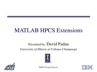
A{1,1} B{1,1} A{1,2} B{2,2} A{1,3} B{3,3} A{1,4} B{4,4} A{2,2} B{2,1} A{2,3} B{3,2} A{2,4} B{4,3} A{2,1} B{1,4} A{3,3} B{3,1} A{3,4} B{4,2} A{3,1} B{1,3} A{3,2} B{2,4} A{4,4} B{4,1} A{4,1} B{1,2} A{4,2} B{2,3} A{4,3} B{3,4} Using HTAs to Represent Data Distribution and Parallelism Cannon’s Algorithm
A{1,1} B{1,1} A{1,2} B{2,2} A{1,3} B{3,3} A{1,4} B{4,4} A{2,2} B{2,1} A{2,3} B{3,2} A{2,4} B{4,3} A{2,1} B{1,4} A{3,3} B{3,1} A{3,4} B{4,2} A{3,1} B{1,3} A{3,2} B{2,4} A{4,4} B{4,1} A{4,1} B{1,2} A{4,2} B{2,3} A{4,3} B{3,4}
A{1,2} B{1,1} A{1,3} B{2,2} A{1,4} B{3,3} A{1,1} B{4,4} A{2,3} B{2,1} A{2,4} B{3,2} A{2,1} B{4,3} A{2,2} B{1,4} A{3,4} B{3,1} A{3,1} B{4,2} A{3,2} B{1,3} A{3,3} B{2,4} A{4,1} B{4,1} A{4,2} B{1,2} A{4,3} B{2,3} A{4,4} B{3,4}
A{1,2} B{2,1} A{1,3} B{3,2} A{1,4} B{4,3} A{1,1} B{1,4} A{2,3} B{3,1} A{2,3} B{4,2} A{2,4} B{1,3} A{2,1} B{2,4} A{3,3} B{4,1} A{3,4} B{1,2} A{3,1} B{2,3} A{3,2} B{3,4} A{4,4} B{1,1} A{4,1} B{2,2} A{4,2} B{3,3} A{4,3} B{4,4}
Cannnon’s Algorithm in MATLAB with HPCS Extensions a=hta(A,{1:SZ/n:n,1:SZ/n:n},[n n]); b=hta(B,{1:SZ/n:n,1:SZ/n:n},[n n]); c=hta(n,n,[n n]); c{:,:} = zeros(p,p); for i=2:n a{i,:} = circshift(a{i,:}, [0 -1]); b{:,i} = circshift(b{:,i}, [-1 0]); end for k=1:n c = c + a * b; a = circshift(a,[0 -1]); b = circshift(b,[-1 0]); end
Cannnon’s Algorithm in C + MPI for (km = 0; km < m; km++) { char *chn = "T"; dgemm(chn, chn, lclMxSz, lclMxSz, lclMxSz, 1.0, a, lclMxSz, b, lclMxSz, 1.0, c, lclMxSz); MPI_Isend(a, lclMxSz * lclMxSz, MPI_DOUBLE, destrow, ROW_SHIFT_TAG, MPI_COMM_WORLD, &requestrow); MPI_Isend(b, lclMxSz * lclMxSz, MPI_DOUBLE, destcol, COL_SHIFT_TAG, MPI_COMM_WORLD, &requestcol); MPI_Recv(abuf, lclMxSz * lclMxSz, MPI_DOUBLE, MPI_ANY_SOURCE, ROW_SHIFT_TAG, MPI_COMM_WORLD, &status); MPI_Recv(bbuf, lclMxSz * lclMxSz, MPI_DOUBLE, MPI_ANY_SOURCE, COL_SHIFT_TAG, MPI_COMM_WORLD, &status); MPI_Wait(&requestrow, &status); aptr = a; a = abuf; abuf = aptr; MPI_Wait(&requestcol, &status); bptr = b; b = bbuf; bbuf = bptr; }
The SUMMA Algorithm (1 of 6) Use now the outer-product method (n2-parallelism) Interchanging the loop headers of the loop in Example 1 produce: for k=1:n for i=1:n for j=1:n C{i,j}=C{i,j}+A{i,k}*B{k,j} end end end To obtain n2 parallelism, the inner two loops should take the form of a block operations: for k=1:n C{:,:}=C{:,:}+A{:,k} B{k,:}; end Where the operator represents the outer product operations
The SUMMA Algorithm (2 of 6) • The SUMMA Algorithm C A B b11 b12 Switch Orientation -- By using a column of A and a row of B broadcast to all, compute the “next” terms of the dot product a11 a21 a11b11 a11b12 a21b11 a21b12
The SUMMA Algorithm (3 of 6) c{1:n,1:n} = zeros(p,p); % communication for i=1:n t1{:,:}=spread(a(:,i),dim=2,ncopies=N); % communication t2{:,:}=spread(b(i,:),dim=1,ncopies=N); % communication c{:,:}=c{:,:}+t1{:,:}*t2{:,:}; % computation end
Matrix Multiplication with Columnwise Block Striped Matrix for i=0:p-1 block(i) =[ i*n/p : (i-1)*n/p-1 ]; end for i=0:p-1 M{i} = A(:,block(i)); v{i} = b(block(i)); end forall j=0:p-1 c{j} =M{i}*v{j}; end forall i=0:p-1;j=0:p-1 d{i}(j) = c{j}(i) end forall i=0:p-1 b{i} = sum(d{i}) end
Flattening • Elements of an HTA are referenced using a tile index for each level in the hierarchy followed by an array index. Each tile index tuple is enclosed within {}s and the array index is enclosed within parentheses. • In the matrix multiplication code, C{i,j}(3,4) would represent element 3,4 of submatrix i,j. • Alternatively, the tiled array could be accessed as a flat array as shown in the next slide. • This feature is useful when a global view of the array is needed in the algorithm. It is also useful while transforming a sequential code into parallel form.
C{1,1}(1,1) C(1,1) C{1,2}(1,1) C(1,5) C{1,1}(1,2) C(1,2) C{1,1}(1,3) C(1,3) C{1,1}(1,4) C(1,4) C{1,2}(1,2) C(1,6) C{1,2}(1,3) C(1,7) C{1,2}(1,4) C(1,8) C{1,1}(2,1) C(2,1) C{1,1}(2,2) C(2,2) C{1,1}(2,3) C(2,3) C{1,1}(2,4) C(2,4) C{1,2}(2,1) C(2,5) C{1,2}(2,2) C(2,6) C{1,2}(2,3) C(2,7) C{1,2}(2,4) C(2,8) C{1,1}(3,1) C(3,1) C{1,2}(3,1) C(3,5) C{1,1}(3,2) C(3,2) C{1,1}(3,3) C(3,3) C{1,1}(3,4) C(3,4) C{1,2}(3,2) C(3,6) C{1,2}(3,3) C(3,7) C{1,2}(3,4) C(3,8) C{1,1}(4,1) C(4,1) C{1,1}(4,2) C(4,2) C{1,1}(4,3) C(4,3) C{1,1}(4,4) C(4,4) C{1,2}(4,1) C(4,5) C{1,2}(4,2) C(4,6) C{1,2}(4,3) C(4,7) C{1,2}(4,4) C(4,8) C{2,1}(1,1) C(5,1) C{2,2}(1,1) C(5,5) C{2,1}(1,2) C(5,2) C{2,1}(1,3) C(5,3) C{2,1}(1,4) C(5,4) C{2,2}(1,2) C(5,6) C{2,2}(1,3) C(5,7) C{2,2}(1,4) C(5,8) C{2,1}(2,1) C(6,1) C{2,1}(2,2) C(6,2) C{2,1}(2,3) C(6,3) C{2,1}(2,4) C(6,4) C{2,2}(2,1) C(6,5) C{2,2}(2,2) C(6,6) C{2,2}(2,3) C(6,7) C{2,2}(2,4) C(6,8) C{2,1}(3,1) C(7,1) C{2,2}(3,1) C(7,5) C{2,1}(3,2) C(7,2) C{2,1}(3,3) C(7,3) C{2,1}(3,4) C(7,4) C{2,2}(3,2) C(7,6) C{2,2}(3,3) C(7,7) C{2,2}(3,4) C(7,8) C{2,1}(4,1) C(8,1) C{2,1}(4,2) C(8,2) C{2,1}(4,3) C(8,3) C{2,1}(4,4) C(8,4) C{2,2}(4,1) C(8,5) C{2,2}(4,2) C(8,6) C{2,2}(4,3) C(8,7) C{2,2}(4,4) C(8,8) Two Ways of Referencing the Elements of an 8 x 8 Array.
Status • We have completed the implementation of practically all of our initial language extensions (for IBM SP-2 and Linux Clusters). • Following the toolbox approach has been a challenge, but we have been able to overcome all obstacles.
Jacobi Relaxation while dif > epsilon v{2:,:}(0,:) = v{:n-1,:}(p,:); % communication v{:n-1,:} (p+1,:) = v{2:,:} (1,:); % communication v{:,2:} (:,0) = v{:,1:n-1}(:,p); % communication v{:, :n-1}(:,p+1) = v{:,2:}(:,1); % communication u{:,:}(1:p,1:p) = a * (v{:,:} (1:p,0:p-1) + v{:,:} (0:p-1,1:p)+ v{:,:} (1:p,2:p+1) + v{:,:} (2:p+1,1:p)) ; %computation dif=max(max( abs ( v – u ) )); v = u ; end
Sparse Matrix Vector Product P1 P2 P3 b A (Distributed) (Replicated) P4
Sparse Matrix Vector Product HTA Implementation c = hta(a, {dist, [1]}, [4 1]); v = hta(4,1,[4 1]); v{:} = b; t = c * v; r = t(:);
Tools • MATLABTM allows user-defined classes • Functions can be written in C, FORTRAN (mex) • Obvious communication tool: MPI • MATLABTM currently provides us both the language and the computation engine both in the client and the servers • Standard MATLABTM extension mechanism: toolbox
MATLABTM Classes • Have constructor, methods • They are standard MATLABTM functions (possibly mex files) that can access the internals of the class • Allow overloading of standard operators and functions • Big problem: no destructors!! • Solution: register created HTAs and apply garbage collection
Architecture MATLABTM MATLABTM Client Server HTA Subsystem HTA Subsystem MPI Interface MPI Interface Mex Functions MATLABTM Functions MATLABTM Functions Mex Functions
HTAs Currently Supported • Dense and sparse matrices • Real and complex double precision • Any number of levels of tiling • HTAs must be either completely empty or completely full • Every tile in an HTA must have the same number of levels of tiling
Communication Patterns • Client • Broadcasts commands & data • Synchronizes servers sometimes • Still, servers can swap tiles following commands issued by client • So in some operations the client is a bottleneck in the current implementation, while in others the system is efficient
Communication Implementation • No MPI collective communications used • Individual messages • Extensive usage of non blocking sends • Every message is a vector of doubles • Internally MATLABTM stores most of its data as doubles • Faster/easier development
Conclusions • We have developed parallel extensions to MATLAB. • It is possible to write highly readable parallel code for both dense and sparse computations with these extensions. • The HTA objects and operations have been implemented as a MATLAB toolbox which enabled their implementation as language extensions.