Download
1 / 54
941 likes | 1.59k Views
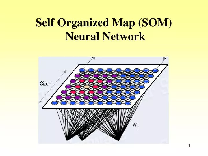
Self Organized Map (SOM) Neural Network. Self Organized Map (SOM). The self-organizing map (SOM) is a method for unsupervised learning , based on a grid of artificial neurons whose weights are adapted to match input vectors in a training set.

E N D
Self Organized Map (SOM) Neural Network
Self Organized Map (SOM) • The self-organizing map (SOM) is a method for unsupervised learning, based on a grid of artificial neurons whose weights are adapted to match input vectors in a training set. • It was first described by the Finnish professor Teuvo Kohonen and is thus sometimes referred to as a Kohonen map. • SOM is one of the most popular neural computation methods in use, and several thousand scientific articles have been written about it. SOM is especially good at producing visualizations of high-dimensional data.
Self Organizing Maps (SOM) • SOM is an unsupervised neural network technique that approximates an unlimited number of input data by a finite set of models arranged in a grid, where neighbor nodes correspond to more similar models. • The models are produced by a learning algorithm that automatically orders them on the two-dimensional grid along with their mutual similarity.
Brain’s self-organization The brain maps the external multidimensional representation of the world into a similar 1 or 2 - dimensional internal representation. That is, the brain processes the external signals in a topology-preserving way Mimicking the way the brain learns, our system should be able to do the same thing.
Why SOM ? • Unsupervised Learning • Clustering • Classification • Monitoring • Data Visualization • Potential for combination between SOM and other neural network (MLP-RBF)
Self Organizing Networks • Discover significant patterns or features in the input data • Discovery is done without a teacher • Synaptic weights are changed according to local rules • The changesaffect a neuron’s immediate environment until a final configurationdevelops
Concept of the SOM. Input space Input layer Reduced feature space Map layer Ba s1 s2 Mn Sr Cluster centers (code vectors) Place of these code vectors in the reduced space Clustering and ordering of the cluster centers in a two dimensional grid
Network Architecture • Two layers of units • Input: n units (length of training vectors) • Output: m units (number of categories) • Input units fully connected with weights to output units • Intralayer (lateral) connections • Within output layer • Defined according to some topology • Not weights, but used in algorithm for updating weights
SOM - Architecture j 2d array of neurons Weights wj1 wj2 wj3 wjn Set of input signals x1 x2 x3 ... xn • Lattice of neurons (‘nodes’) accepts and responds to set of input signals • Responses compared; ‘winning’ neuron selected from lattice • Selected neuron activated together with ‘neighbourhood’ neurons • Adaptive process changes weights to more closely inputs
Measuring distances between nodes • Distances between output neurons will be used in the learning process. • It may be based upon: • Rectangular lattice • Hexagonal lattice • Let d(i,j) be the distance between the output nodes i,j • d(i,j) = 1 if node j is in the first outer rectangle/hexagon of node i • d(i,j) = 2 if node j is in the second outer rectangle/hexagon of node i • And so on..
Each neuron is a node containing a template against which input patterns are matched. • All Nodes are presented with the same input pattern in parallel and compute the distance between their template and the input in parallel. • Only the node with the closest match between the input and its template produces an active output. • Each Node therefore acts like a separate decoder (or pattern detector, feature detector) for the same input and the interpretation of the input derives from the presence or absence of an active response at each location • (rather than the magnitude of response or an input-output transformation as in feedforward or feedback networks).
SOM: interpretation • Each SOM neuron can be seen asrepresenting a cluster containing all the input examples which are mapped to that neuron. • For a given input, the output of SOM is the neuron with weight vector most similar (with respect to Euclidean distance) to that input.
Self-Organizing Networks • Kohonen maps (SOM) • Learning Vector Quantization (VQ) • Principal Components Networks (PCA) • Adaptive Resonance Theory (ART)
Types of Mapping • Familiarity – the net learns how similar is a given new input to the typical (average) pattern it has seen before • The net finds Principal Components in the data • Clustering – the net finds the appropriate categories based on correlations in the data • Encoding – the output represents the input, using a smaller amount of bits • Feature Mapping – the net forms a topographic map of the input
Possible Applications • Familiarity and PCA can be used to analyze unknown data • PCA is used for dimension reduction • Encoding is used for vector quantization • Clustering is applied on any types of data • Feature mapping is important for dimension reduction and for functionality (as in the brain)
Simple Models • Network has inputs and outputs • There is no feedbackfrom the environment no supervision • The network updates the weights following some learning rule, and finds patterns, features or categories within the inputs presented to the network
Unsupervised Learning In unsupervised competitive learning the neurons take part in some competition for each input. The winner of the competition and sometimes some other neurons are allowed to change their weights • In simple competitive learning only the winner is allowed to learn (change its weight). • In self-organizing maps other neurons in the neighborhood of the winner may also learn.
W11 Y1 x1 W12 x2 W22 WP1 Y2 xN WPN YP Simple Competitive Learning N inputs units P output neurons P x N weights
Network Activation • The unit with the highest field hi fires • i* is the winner unit • Geometrically is closest to the current input vector • The winning unit’s weight vector is updated to be even closer to the current input vector
Learning Starting with small random weights, at each step: • a new input vector is presented to the network • all fields are calculated to find a winner • is updated to be closer to the input Using standard competitive learning equ.
Result • Each output unit moves to the center of mass of a cluster of input vectors clustering
Competitive Learning, Cntd • It is important to break the symmetry in the initial random weights • Final configuration depends on initialization • A winning unit has more chances of winning the next time a similar input is seen • Some outputs may never fire • This can be compensated by updating the non winning units with a smaller update
More about SOM learning • Upon repeated presentations of the training examples, the weight vectors of the neurons tend to followthe distribution of the examples. • This results in a topological ordering of the neurons, where neurons adjacent to each other tend to have similar weight vectors. • The input space of patterns is mapped onto a discrete output space of neurons.
SOM – Learning Algorithm • Randomly initialise all weights • Select input vector x = [x1, x2, x3, … , xn] from training set • Compare x with weights wj for each neuron j to • determine winner find unit j with the minimum distance • Update winner so that it becomes more like x, together with the winner’s neighbours for units within the radius according to • Adjust parameters: learning rate & ‘neighbourhood function’ • Repeat from (2) until … ? Note that: Learning rate generally decreases with time:
Example An SOFM network with three inputs and two cluster units is to be trained using the four training vectors: [0.8 0.7 0.4], [0.6 0.9 0.9], [0.3 0.4 0.1], [0.1 0.1 02] and initial weights The initial radius is 0 and the learning rate is 0.5 . Calculate the weight changes during the first cycle through the data, taking the training vectors in the given order. 0.5 0.6 weights to the first cluster unit 0.8
Solution The Euclidian distance of the input vector 1 to cluster unit 1 is: The Euclidian distance of the input vector 1 to cluster unit 2 is: Input vector 1 is closest to cluster unit 1 so update weights to cluster unit 1:
Solution The Euclidian distance of the input vector 2 to cluster unit 1 is: The Euclidian distance of the input vector 2 to cluster unit 2 is: Input vector 2 is closest to cluster unit 1 so update weights to cluster unit 1 again: Repeat the same update procedure for input vector 3 and 4 also.
Neighborhood Function • Gaussian neighborhood function: • dji: lateral distance of neurons i and j • in a 1-dimensional lattice | j - i | • in a 2-dimensional lattice || rj - ri || where rj is the position of neuron j in the lattice.
N13(1) N13(2)
Neighborhood Function • measures the degree to which excited neurons in the vicinity of the winning neuron cooperate in the learning process. • In the learning algorithm is updated at each iteration during the ordering phase using the following exponential decay update rule, with parameters
Degree of neighbourhood Time Distance from winner Neighbourhood function Degree of neighbourhood Distance from winner Time
UPDATE RULE exponential decay update of the learning rate:
y x Illustration of learning for Kohonen maps Inputs: coordinates (x,y) of points drawn from a square Display neuron j at position xj,yj where its sj is maximum 100 inputs 200 inputs 1000 inputs Random initial positions
Two-phases learning approach • Self-organizing or ordering phase. The learning rate and spread of the Gaussian neighborhood function are adapted during the execution of SOM, using for instance the exponential decay update rule. • Convergence phase. The learning rate and Gaussian spread have small fixed values during the execution of SOM.
1000 log (0) Ordering Phase • Self organizing or ordering phase: • Topological ordering of weight vectors. • May take 1000 or more iterations of SOM algorithm. • Important choice of the parameter values. For instance • (n): 0 = 0.1 T2 = 1000 decrease gradually (n) 0.01 • hji(x)(n): 0 big enough T1 = • With this parameter setting initially the neighborhood of the winning neuron includes almost all neurons in the network, then it shrinks slowly with time.
Convergence Phase • Convergence phase: • Fine tune the weight vectors. • Must be at least 500 times the number of neurons in the network thousands or tens of thousands of iterations. • Choice of parameter values: • (n) maintained on the order of 0.01. • Neighborhood function such that the neighbor of the winning neuron contains only the nearest neighbors. It eventually reduces to one or zero neighboring neurons.
Another Self-Organizing Map (SOM) Example • From Fausett (1994) • n = 4, m = 2 • More typical of SOM application • Smaller number of units in output than in input; dimensionality reduction • Training samples i1: (1, 1, 0, 0) i2: (0, 0, 0, 1) i3: (1, 0, 0, 0) i4: (0, 0, 1, 1) Network Architecture Input units: 1 2 Output units: What should we expect as outputs?
What are the Euclidean Distances Between the Data Samples? • Training samples i1: (1, 1, 0, 0) i2: (0, 0, 0, 1) i3: (1, 0, 0, 0) i4: (0, 0, 1, 1)
Euclidean Distances Between Data Samples • Training samples i1: (1, 1, 0, 0) i2: (0, 0, 0, 1) i3: (1, 0, 0, 0) i4: (0, 0, 1, 1) Input units: What might we expect from the SOM? 1 2 Output units:
Input units: Example Details 1 2 Output units: • Training samples i1: (1, 1, 0, 0) i2: (0, 0, 0, 1) i3: (1, 0, 0, 0) i4: (0, 0, 1, 1) • With only 2 outputs, neighborhood = 0 • Only update weights associated with winning output unit (cluster) at each iteration • Learning rate (t) = 0.6; 1 <= t <= 4 (t) = 0.5 (1); 5 <= t <= 8 (t) = 0.5 (5); 9 <= t <= 12 etc. • Initial weight matrix (random values between 0 and 1) Unit 1: Unit 2: d2 = (Euclidean distance)2 = Weight update: Problem: Calculate the weight updates for the first four steps
i1: (1, 1, 0, 0) • i2: (0, 0, 0, 1) • i3: (1, 0, 0, 0) • i4: (0, 0, 1, 1) First Weight Update Unit 1: Unit 2: • Training sample: i1 • Unit 1 weights • d2 = (.2-1)2 + (.6-1)2 + (.5-0)2 + (.9-0)2 = 1.86 • Unit 2 weights • d2 = (.8-1)2 + (.4-1)2 + (.7-0)2 + (.3-0)2 = .98 • Unit 2 wins • Weights on winning unit are updated • Giving an updated weight matrix: Unit 1: Unit 2:
i1: (1, 1, 0, 0) • i2: (0, 0, 0, 1) • i3: (1, 0, 0, 0) • i4: (0, 0, 1, 1) Second Weight Update Unit 1: Unit 2: • Training sample: i2 • Unit 1 weights • d2 = (.2-0)2 + (.6-0)2 + (.5-0)2 + (.9-1)2 = .66 • Unit 2 weights • d2 = (.92-0)2 + (.76-0)2 + (.28-0)2 + (.12-1)2 = 2.28 • Unit 1 wins • Weights on winning unit are updated • Giving an updated weight matrix: Unit 1: Unit 2:
i1: (1, 1, 0, 0) • i2: (0, 0, 0, 1) • i3: (1, 0, 0, 0) • i4: (0, 0, 1, 1) Third Weight Update Unit 1: Unit 2: • Training sample: i3 • Unit 1 weights • d2 = (.08-1)2 + (.24-0)2 + (.2-0)2 + (.96-0)2 = 1.87 • Unit 2 weights • d2 = (.92-1)2 + (.76-0)2 + (.28-0)2 + (.12-0)2 = 0.68 • Unit 2 wins • Weights on winning unit are updated • Giving an updated weight matrix: Unit 1: Unit 2:
i1: (1, 1, 0, 0) • i2: (0, 0, 0, 1) • i3: (1, 0, 0, 0) • i4: (0, 0, 1, 1) Fourth Weight Update Unit 1: Unit 2: • Training sample: i4 • Unit 1 weights • d2 = (.08-0)2 + (.24-0)2 + (.2-1)2 + (.96-1)2 = .71 • Unit 2 weights • d2 = (.97-0)2 + (.30-0)2 + (.11-1)2 + (.05-1)2 = 2.74 • Unit 1 wins • Weights on winning unit are updated • Giving an updated weight matrix: Unit 1: Unit 2:
Applying the SOM Algorithm Data sample utilized ‘winning’ output unit After many iterations (epochs) through the data set: Unit 1: Unit 2: Did we get the clustering that we expected?
Training samples • i1: (1, 1, 0, 0) • i2: (0, 0, 0, 1) • i3: (1, 0, 0, 0) • i4: (0, 0, 1, 1) What clusters do thedata samples fall into? Weights Input units: Unit 1: Unit 2: 1 2 Output units:
Training samples • i1: (1, 1, 0, 0) • i2: (0, 0, 0, 1) • i3: (1, 0, 0, 0) • i4: (0, 0, 1, 1) Weights Unit 1: Solution Input units: Unit 2: 1 2 Output units: • Sample: i1 • Distance from unit1 weights • (1-0)2 + (1-0)2 + (0-.5)2 + (0-1.0)2 = 1+1+.25+1=3.25 • Distance from unit2 weights • (1-1)2 + (1-.5)2 + (0-0)2 + (0-0)2 = 0+.25+0+0=.25 (winner) • Sample: i2 • Distance from unit1 weights • (0-0)2 + (0-0)2 + (0-.5)2 + (1-1.0)2 = 0+0+.25+0 (winner) • Distance from unit2 weights • (0-1)2 + (0-.5)2 + (0-0)2 + (1-0)2 =1+.25+0+1=2.25 d2 = (Euclidean distance)2 =
Training samples • i1: (1, 1, 0, 0) • i2: (0, 0, 0, 1) • i3: (1, 0, 0, 0) • i4: (0, 0, 1, 1) Weights Unit 1: Solution Input units: Unit 2: 1 2 Output units: • Sample: i3 • Distance from unit1 weights • (1-0)2 + (0-0)2 + (0-.5)2 + (0-1.0)2 = 1+0+.25+1=2.25 • Distance from unit2 weights • (1-1)2 + (0-.5)2 + (0-0)2 + (0-0)2 = 0+.25+0+0=.25 (winner) • Sample: i4 • Distance from unit1 weights • (0-0)2 + (0-0)2 + (1-.5)2 + (1-1.0)2 = 0+0+.25+0 (winner) • Distance from unit2 weights • (0-1)2 + (0-.5)2 + (1-0)2 + (1-0)2 = 1+.25+1+1=3.25 d2 = (Euclidean distance)2 =