Download
1 / 18
180 likes | 308 Views
Self Organized Maps (SOM). CUNY Graduate Center December 15 Erdal Kose. Outlines. Define SOMs Application Areas Structure Of SOMs (Basic Algorithm) Learning Algorithm Simulation and Results Conclusion References. SOMs.

E N D
Self Organized Maps (SOM) CUNY Graduate Center December 15 Erdal Kose
Outlines • Define SOMs • Application Areas • Structure Of SOMs (Basic Algorithm) • Learning Algorithm • Simulation and Results • Conclusion • References
SOMs • The best know and most popular model of Self-organizing networks is the topology-preserving map proposed by TeuvoKohonen, known as Kohanen networks • They provide a way of representing multidimensional data in much lower dimensional space, such as one or two dimensions.
Applications • Image compression • Data minding • Bibliographic classification • Image browsing systems • Medical Diagnosis • Speech recognition • Clustering
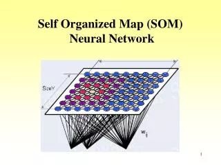
Structure of SOM • A self organized map consists of components called nodes • Associated with each node is a weight vector of the same dimension as the input data vectors • and a position in the map space • The usual arrangement of nodes is a regular spacing in a hexagonal or rectangular grid
Learning Algorithm • Each node's weights are initialized. • A vector is chosen at random from the set of training data and presented to the lattice. • Every node is examined to calculate which one's weights are most like the input vector. The winning node is commonly known as the Best Matching Unit (BMU). • The radius of the neighborhood of the BMU is now calculated. This is a value that starts large, typically set to the 'radius' of the lattice, but diminishes each time-step. Any nodes found within this radius are deemed to be inside the BMU's neighborhood. • Each neighboring node's (the nodes found in step 4) weights are adjusted to make them more like the input vector. The closer a node is to the BMU, the more its weights get altered. • Repeat step 2 for N iterations. http://www.ai-junkie.com/ann/som/som2.html
The learning Algorithm in detail • Random initialization means simply that random values are assigned to weight vectors. This is the case if nothing or little is known about the input data at the time of the initialization • In one training step, one sample vector is drawn randomly from the input data set , This vector is fed to all units in the network and a similarity measure is calculated between the input data sample and all the weight vectors
Cont. • The best matching unit: The Euclidian distance • After finding the best-matching unit, units in the SOM are updated
Cont.. • The neighborhood function includes the learning rate function which is a decreasing function of time and the function that dictates the form of the neighborhood function.
Adjusting the Weights • Every node within the best matching unit’s (BMU) neighborhood (including the BMU) has its weight vector adjusted according to the following equation: W(t+1)=W(t)+α(t)(V(t)-W(t) • Where trepresents the time-step and α is the learning rate, which decreases with time. • Basically, what this equation is saying, is that the new adjusted weight for the node is equal to the old weight (W), plus a fraction of the difference (α) between the old weight and the input vector (V)
Visulization • World Poverty Map • A SOM has been used to classify statistical data describing various quality-of-life factors such as state of health, nutrition, educational services etc.
Conclusion • The Kohonen Feature Map was first introduced by finnish professor TeuvoKohonen (University of Helsinki) in 1982. • The "heart" of this type of networks is the feature map • a neuron layer where neurons are organizing themselves according to certain input values. • They could learn without supervision
References • A growing Self-Organizing Algorithm for Dynamic Clustering Ryuji Ohta, Toshimichi Saito Hosei university ,Japan (IEEE 2001) • A Self-Organization Model of Feature Columns and Face Responsive Neurons in the Temporal ContexTakashie Takahashi, Tako Kurita National Institute of Advanced Industrial Science and Technology (2001 IEEE) • http://www.cis.hut.fi/projects/ica/cocktail/cocktail_en.cgi • http://www.cis.hut.fi/~jhollmen/dippa/node9.html • http://www.ai-junkie.com/ann/som/som1.html • http://www.borgelt.net/doc/somd/somd.html • http://www.nnwj.de/sample-applet.html • http://fbim.fh-regensburg.de/~saj39122/jfroehl/diplom/e-sample.html