Download
1 / 22
1.2k likes | 3.42k Views
5. Dynamic behavior of First-order and Second-order Systems. Contents 1. Standard Process Inputs. 2. Response of First-Order Systems. 3. Response of Integrating Process. 4. Response of Second-Order Systems.

E N D
5. Dynamic behavior of First-order and Second-order Systems • Contents 1. Standard Process Inputs. 2. Response of First-Order Systems. 3. Response of Integrating Process. 4. Response of Second-Order Systems. • In this chapter, we learn how process respond to typical changes in some of input changes. • Two categories in process inputs. 1. Inputs that can be manipulated to control the process. 2. Inputs that are not manipulated, classified as disturbance or load variable.
5.1 Standard Process Inputs - Six important types of input changes. 1. Step input. 2. Ramp input. Figure 5.1. Step input. Figure 5.2. Ramp input.
3. Rectangular Pulse. or Where is unit step function. 4. Sinusoidal input. Figure 5.3. Rectangular Pulse.
5. Impulse input. • It has the simplest Laplace transform, but it is not a realistic input signal. Because to obtain an impulse input, it is necessary to inject amount of energy or material into a process in an infinitesimal length of time. 6. Random inputs. • Many process inputs change with time in such a complex manner that it is not possible to describe them as deterministic functions of time. If an input exhibits apparently random fluctuation, it is convenient to characterize it in statistical terms.
5.2 Response of First-Order Systems - General first-order transfer function. Where is the process gain and is the time constant. • Find and for some particular input . 1. Step response. Figure 5.4. Step response.
A first-order system dose not respond instantaneously to a sudden change in its input and that after a time interval equal to the process time constant ( ), the process response is still only 63.2% complete. • Theoretically the process output never reaches the new steady-state value; it dose approximate the new value when t equals 3 to 5 process time constants.
2. Ramp response. • Interesting property for large values of time( ). • After an initial transient period, the ramp input yields a ramp output with slope equal to , but shifted in time but the process time constant . Figure 5.5. Ramp response. - comparison of input and output.
3. Sinusoidal response. • By trigonometric identities. Where . • Trigonometric identities. Where .
Phase lag • Remarks 1. In both (5.21) and (5.22), the exponential term goes to zero as leaving a pure sinusoidal response. • Frequency Response ! (will be discussed later). 2. Since , amplitude is less than output f or input . Amplitude attenuation ! Figure 5.6. Typical sinusoidal response.
5.3 Response of Integrating Process Units • What is an ‘Integrating Process’? ; The process which has integrating unit( ) in its transfer function. • Open-loop unstable process(Non-self-regulating process). • A process that cannot reach a new steady state when subjected to step changes in inputs is called ‘Open-loop unstable process’ or ‘Non-self-regulating process’. • Which process is an integrating process? Figure 5.7. Liquid level system with a pump(a) or valve(b).
Answer )(a) is the integrating process! The flowrate of the effluent stream (b) increase automatically if the level increase. Therefore, the influent flowrate is increased then the level will increase and the effluent flowrate also increased up to the influent flowrate so the level will converge. • Liquid level system with a valve is a stable(or self-regulating) process. But, in (a), regardless of the level, the effluent flowrate is constant due to the pump. So, if the influent flowrate is bigger than the effluent stream the level always increase, vice versa. That is, the difference between the influent flowrate and the effluent flowrate is integrated to the process output(the level). • Liquid level system with a pump is a unstable(or non-self-regulating) process.
Example Where is independent of . Integrating process ! Figure 5.8. Liquid level system with a pump.
5.4 Response of Second-Order Systems • A second order transfer function can arise physically, • Two first-order processes are connected in series. Figure 5.9. Two first-order systems in series yield an overall second-order system. • A second-order differential equation process model is transformed.
Where is the process gain. is the time constant which determines the speed of response of the system. is the damping factor which provides a measure of the amount of damping in the system, that is, the degree of oscillation in a process response after a perturbation. • Standard form of the second-order transfer function.
Three important subcases. • Denominator of (5.28); • Roots ; • ; unstable second-order system that would have an unbounded response to any input.
Case a. , root are real and distinct:Overdamped. Case b. , double root: Critically damped. 1. Step response. Case c. , complex root: Underdamped. Where
Remarks • Responses exhibiting oscillation and overshoot( ) are obtained only for values of less than one. • Large value of yield a sluggish response. • The faster response without overshoot is obtained for critically damped case( ). Figure 5.10. Step response of critically-damped and overdamped(a), and underdamped(b) second-order processes.
A number of terms that describe the dynamics of underdamped processes. 1. Rise time( ) is the time the process output takes to first reach the new steady-state value. 2. Time to first peak( ) is the time required for the output to reach its first maximum value. 3. Settling time( ) is defined as the time required for the process output reach and remain inside a band whose width is equal to of the total change in . 4. Overshoot. 5. Decay ratio. 6. Period of Oscillation( ) is the time between two successive peaks or two successive valleys of the responses. Figure 5.11. Performance characteristics for the step response.
Overshoot. • Rise time. • Time to first peak.
Decay ratio. • Period of oscillation. Figure 5.12. Relation between some performance characteristics of an underdamped second-order process and the process damping coefficient.
2. Sinusoidal response. As , the first and second terms vanish. Thus the output for large values of time is obtained as follows. Where • Amplitude ratio • Normalized amplitude ratio
For , there is no maximum. • The maximum value of can be found by differentiating (5.45) with respect to . • At high frequency, the output is well damped. • At low frequency, the output is not damped well. Figure 5.13. Sinusoidal response amplitude of a second-order system after exponential terms have become negligible.