Download
1 / 33
330 likes | 335 Views
MICROWAVE REMOTE SENSING AND. SST FROM PASSIVE MICROWAVE OBSERVATIONS. MICROWAVE REMOTE SENSING. WHY MW REMOTE SENSING?. WHY MW REMOTE SENSING?. RESULTS FROM ISCCP. The global annual mean cloud amount is about 66.7% and exhibits little variation from month to month over the whole 25 yrs.

E N D
MICROWAVE REMOTE SENSING AND SST FROM PASSIVE MICROWAVE OBSERVATIONS
WHY MW REMOTE SENSING? RESULTS FROM ISCCP • The global annual mean cloud amount is about 66.7% and exhibits little variation from month to month over the whole 25 yrs. • ISCCP record, the global annual mean cloud amount has undergone a slow cycle, apparently associated with E1 Nino occurrences, with an amplitude of + 4%. • The mean annual Southern Hemisphere cloud amount is almost 6% larger than the mean Northern Hemisphere cloud amount • The mean western hemisphere cloud amount is a little more than 4% larger than the eastern hemisphere cloud average cloud amount over ocean and land and form the difference in hemispheric land fractions. • The mean annual ocean cloud amount is about 23% larger than the land cloud amount (the ISCCP results probably overestimate this difference by 5%-10%).
MICROWAVE REMOTE SENSING • Microwave instruments collect data in all weather conditions because microwaves penetrate most cloud cover. • Microwave remote sensing application areas include: ocean storm reconnaissance; observation of snow- and ice-covered regions; monitoring of land and sea surface temperature; measurement of precipitation, clouds, and water vapor; and global climate monitoring. • The microwave frequencies for meteorological observation fall in the range from about 5 to 200 GHz or 6 to 0.15 cm. • Active sensors send a microwave signal to the earth and measure the return signal. • Passive sensors detect both natural and anthropogenic microwave emissions from earth's atmosphere and surface
MICROWAVE REMOTE SENSING • Microwave imagers produce two-dimensional images of brightness temperature and a variety of derived products. • Microwave sounders produce three-dimensional representations of atmospheric temperature and moisture. • Modern microwave imagers and sounders can produce both imaging and sounding data. • Currently, there are numerous active and passive microwave sensors flying on different polar-orbiting satellites. • The NPOESS satellite constellation will carry two passive microwave sensors: CMIS (Conical Microwave Imager Sounder is primarily an imager, but can also provide sounding products ) and ATMS (The Advanced Technology Microwave Sounder primarily provides temperature and moisture profiles, but it can also be used as an imager)
Active Microwave Radiometers Active microwave radiometers have an onboard power supply used to send periodic energy pulses toward the earth and measure the signal return. Weather radars located on the earth’s surface, such as Doppler radar, work in a similar way.
Passive Microwave Radiometer A passive microwave radiometer sends no pulses out toward the earth. Instead, the sensor receives radiation emitted from the earth/atmosphere system, including precipitation, water vapor, clouds, and the surface. Several passive microwave sensors are currently providing data for monitoring weather and the Earth's surface. CMIS and ATMS are the passive sensors scheduled to provide data continuity and new observing capabilities in the NPOESS era.
Microwave Imaging and Sounding . • There are two different classes of microwave instruments flown on polar satellites: imagers and sounders • Microwave imagers primarily produce two dimensional products, often displayed as images or maps. Sea surface temperature plots are an example of this data type.
Microwave Sounders • Produce data that represent the three-dimensional structure of atmospheric temperature and moisture • These data are usually assimilated into numerical models
SST FROM PASSIVE MW OBSERVATIONS • Passive MW Radiometers function the same way as IR radiometers • Observe thermal radiation emitted MW part of the spectrum by • Sea surface • Atmosphere • Radiation reflected by sea surface from atmospheric downward &solar emission • At MW wavelength, there is no scattering by aerosols, haze, dust or water particles in clouds • Liquid water in the form of rain and ice at higher frequencies do scatter radiation
DIS-ADVANTAGES OF MW SENSORS • Thermal emission is very weak and hence signal received at sensor is weak • Need large FOV to reduce noise level (coarser resolution) • The emissivity of sea surface is low (typically 0.3 ) • The emissivity varies with the dielectric property of sea water and surface roughness • The dielectric property of sea water varies with • Temp • Salinity • EM frequency • Need multichannel observations of not only the SST, but also about the ocean salinity and the roughness (sea state)
Thermal Emission in MW • It is controlled by Planck’s Radiation law which can be written as : At microwave frequencies, for temperature encountered on the Earth and in its atmosphere, c2/T << 1 Therefore, exp(c2/T) 1 + (c2/T) The Planck’s function then becomes
ATMOSPHERIC AND SOLAR RADIATION EFFECTS • In MW region, it is customary to divide radiance values by (c1/c2)-4 and the quotient is referred as Brightness Temperature • The Brightness Temp Tb(θ,) as viewed by sensor contains contributions from sources other than the Sea Surface • The RTE gives the TB measured by the Satellite Radiometer as given below :- TB() = Tu ()+ (0,H)x{Ts+ (1- )Td + (1- ) (,0)Tc } Where, Tu is upward propagating radiance is the atmospheric Transmissivity Ts is Surface Temperature Tdis Downward propagating radiance from the atmosphere Tc is extraterrestrial radiation reflected from surface
CONTRIBUTION TO MW RADIATION a - Signal emitted by Sea Surface b – Downward atmospheric emission c - Cosmic radiation d – Direct upward atmospheric emission
The various terms to be evaluated in the above equation are Total absorption coefficient due to water vapour, cloud liquid water content and oxygen
The equation assumes specular reflection at ocean surface • It was numerically evaluated by dividing the atmosphere in to thin layers, each with specified temp, pressure and humidity • Cloud layers were introduced at various altitudes by specifying cloud top, cloud bottom temperature and liquid water density according to simulated cloud statistics. • Within cloud layers watervapour was added to the profiles to increase the RH to 100%.
Solar contribution to the radiation can be ignored in the MW range as solar radiation peaks at shortwave and fall of at longer wave length. • As with IR, it is not possible to predict the value of as this depends on atmospherically variable quantities such as water vapour, cloud liquid water content, rainfall and oxygen concentration and it is highly dependant on Frequency
CALCULATIONS OF EMMISIVITY • The important parameters involved in simulation of BT (TB) are:- • Emissivity • Total Atmospheric Absorption • New Advances in calculations of emissivity are given by Pandey et al (1982) and Gairola et al 1985 • This emissivity model is applicable for frequency range below 40GHz and wind speed below 25 m/sec • In the presence of roughness and foam the polarised emmisivity of sea surface is given by • p = (sp +Δrp )(1-F) +fp F • Δrpand fp are contributions to emissivity due to surface roughness and foam respectively • F is the effective Fractional foam coverage ( varies from 0 to 1)
CALCULATIONS OF TOTAL ATMOSPHERIC ABSORPTION • Water vapour absorbs in MW region. • WV has a weak and absorption line at 22.235GHz • For atmospheric oxygen, the coefficient incorporates a function of spectral line strength and shape of the absorption spectrum • The absorption in clouds is proportional to its liquid water content. It also incorporates the dielectric properties of water. The values of these parameter is determined as per the result of Hollinger(1973) • Based on the above formulations of the absorption coefficient and emmisivity the main components of the RTE can be computed
ATMOSPHERIC WINDOWS 0.3 - 1.1um 3.0 – 5.0um 2.0 – 2.4um 8.0 – 14.0um > 0.6 Cm 1.5 - 1.8um Absorption Bands in MW Watervapour : 22.2 GHz and 183GHz Oxygen : 60GHz(single line) and 118.7GHz(band)
CALCULATIONS OF TOTAL ATMOSPHERIC ABSORPTION • The RT Equation does not offer the possibility of direct calculation, although it enables different atmospheric composition types to be modeled • This helps in formulation of empirical algorithm to retrieve ocean and atmospheric variables from multi-spectral MW measurements. • 2-10GHz is best for surface viewing • Below this Galactic contribution is strong • Above it correction required for water vapour and oxygen becomes large • Rain remains a problem in 2-10GHz
CONTRIBUTION TO ANTENNA TEMPERATURE FROM ABSORPTION AND GALACTIC BACKGROUND
RETRIEVAL OF SST AND SWS • To retrieve a given geo physical parameter from multiwave length measurements using regression approach • Generation of data base of geo physical parameter and TB (using RTE) • The parameter P is expressed as linear combination of BTs. • P = Ao + An TB • The SST retrieval equation given by Pandey & Kakar(1982) uses a 2 Step statistical techniq-ue based on Regression by Leaps & Bounds to select the best set of radiometric channels
RETRIEVAL OF SST AND SWS • Based on sensitivity studies, for surface parameters more weightage to be given to those channels which are most sensitive to surface parameters and less sensitive to atmospheric parameter • To reduce the effects of non-linearity, use a function of TB than TB it self • The most commonly accepted Logarithmic differential function is F(TB)=ln(280K-TB) • The above function is also used by Gairola et al for atmospheric water component retrieval
SMMR: SEASAT AND NIMBUS-7 • The Scanning Multifrequency Microwave radiometer(SMMR) was flown on Sea Sat (1978) and Nimbus-7 (1983) • The frequencies were 6.63,10.69,18,21 and 37 GHz (both H & V polarisation) • There are 10 diff BTs corresponding to both vertical and horizontal polarisation from which an algorithm was constructed • The resolution is limited to the lowest frequency • The SST retrieval depends on water vapour, cloud liquid water and wind • Hence wind speed is estimated first before estimating SST
SST FROM MSMR:IRS – P4 • IRS-P4(Oceansat-1)The eighth satellite built in India under the indigenous Indian Remote Sensing Satellite programme was successfully launched on May,26,1999 • IRS-P4 carries two sensors onboard, Ocean Color Monitor (OCM) and Multi-frequency Scanning Microwave Radiometer (MSMR). • Orbit Polar, Sun synchronous Altitude 720 km Inclination 98.38 deg Local Time Noon +/- 20 minutes in descending node