Download
1 / 14
140 likes | 155 Views
MESB374 System Modeling and Analysis System Stability and Steady State Response. Stability. where the derivatives of all states are zeros. Stability Concept Describes the ability of a system to stay at its equilibrium position in the absence of any inputs.

E N D
MESB374 System Modeling and AnalysisSystem Stability and Steady State Response
Stability where the derivatives of all states are zeros • Stability Concept Describes the ability of a system to stay at its equilibrium position in the absence of any inputs. • A linear time invariant (LTI) system is stable if and only if (iff) its free response converges to zero for all ICs. Ex: Pendulum Ball on curved surface valley plateau hill inverted pendulum simple pendulum
y y t t TF: TF: Pole: Pole: Examples (stable and unstable 1st order systems) Q: free response of a 1st order system. Q: free response of a 1st order system.
Absolutely Stable Unstable Relative Stability (gain/phase margin) Marginally stable/``unstable’’ Stability of LTI Systems • Stability Criterion for LTI Systems Im Re Complex (s-plane)
Stability of LTI Systems • Comments on LTI Stability • Stability of an LTI system does not depend on the input (why?) • For 1st and 2nd order systems, stability is guaranteed if all the coefficients of the characteristic polynomial are positive (of same sign). • Effect of Poles and Zeros on Stability • Stability of a system depends on its poles only. • Zeros do not affect system stability. • Zeros affect the specific dynamic response of the system.
System Stability (some empirical guidelines) • Passive systems are usually stable • Any initial energy in the system is usually dissipated in real-world systems (poles in LHP); • If there is no dissipation mechanisms, then there will be poles on the imaginary axis • If any coefficients of the denominator polynomial of the TF are zero, there will be poles with zero RP • Active systems can be unstable • Any initial energy in the system can be amplified by internal source of energy (feedback) • If all the coefficients of the denominator polynomial are NOT the same sign, system is unstable • Even if all the coefficients of the denominator polynomial are the same sign, instability can occur (Routh’s stability criterion for continuous-time system)
In Class Exercises (1) Obtain TF of the following system: (2) Plot the poles and zeros of the system on the complex plane. (3) Determine the system’s stability. (1) Obtain TF of the following system: (2) Plot the poles and zeros of the system on the complex plane. (3) Determine the system’s stability. TF: Poles: Poles: Zeros: Zero: Img. Img. Stable Real Real Marginally Stable
Example EOM: Equilibrium position: Inverted Pendulum (1) Derive a mathematical model for a pendulum. (2) Find the equilibrium positions. (3) Discuss the stability of the equilibrium positions. Assumption: is very small Linearized EOM: Characteristic equation: Poles: Img. Unstable Real
Example (Simple Pendulum) EOM: Equilibrium position: How do the positions of poles change when K increases? (root locus) Assumption: is very small Linearized EOM: Characteristic equation: Poles: Img. Img. Img. stable stable stable Real Real Real
Transient and Steady State Response Let’s find the total response of a stable first order system: Ex: to a ramp input: with I.C.: - total response - PFE
Transient and Steady State Response In general, the total response of a STABLE LTI system to a input u(t) can be decomposed into two parts where • Transient Response • contains the free response of the system plus a portion of forced response • will decay to zero at a rate that is determined by the characteristic roots (poles) of the system • Steady State Response • will take the same (similar) form as the forcing input • Specifically, for a sinusoidal input, the steady response will be a sinusoidal signal with the same frequency as the input but with different magnitude and phase.
Transient and Steady State Response Let’s find the total response of a stable second order system: Ex: to a sinusoidal input: with I.C.: - total response - PFE
Steady State Response • Final Value Theorem (FVT) Given a signal’s LT F(s), if all of the poles of sF(s) lie in the LHP, then f(t) converges to a constant value as given in the following form Ex. A linear system is described by the following equation: (1). If a constant input u=5 is applied to the sysetm at time t=0, determine whether the output y(t) will converge to a constant value? (2). If the output converges, what will be its steady state value? • We did not consider the effects of IC since • it is a stable system • we are only interested in steady state response
Steady State Response Given a general n-th order stable system Transfer Function Free Response Steady State Value of Free Response (FVT) In SS value of a stable LTI system, there is NO contribution from ICs.