Download
1 / 61
610 likes | 778 Views
Electrostatic potential determined from electron diffraction data. Anatoly Avilov Shubnikov Institute of Crystallography of Russian academy of sciences, Moscow. Strong interaction with substances.

E N D
Electrostatic potential determined from electron diffraction data Anatoly Avilov Shubnikov Institute of Crystallography of Russian academy of sciences, Moscow
Strong interaction with substances. In the age of nanoscience, there is an urgent need for a method of rapidly solvingnew, inorganic nanostructured materials. Many are fine-grained, with light elements crystallites, thin films which cannot be solved by XRD. Scattering on the electrostatic potential, possibility to reconstruct the potential from ED experiments ED is very sensitive to ionicity, so study of bonding More easy than XRD the localization of light atoms in the presence of heavy ones, solvable problems of hydrogen localization Great intensity of the signal Challenge of electron crystallography
GENERAL for modern SA: Investigation of crystal structure and properties - one of the most important problems of physics and chemistry of solids. Contents of this is changing as development of experimental techiques and theoretical presentations. Study of the features of distribution of ED and inner crystalline field and establishment of their connection with physical properties is one of the major question of modern SA.
Electron diffraction structureanalysis (EDSA) What is it?
EDSA of thin polycrystalline films - advantages Wide beam (100-400 mkm), great amount of micro-crystals in irradiated area - special types of DP-s. Possibly to extract from one DP sufficiently full (3-dim.) set of structure amplitudes. Detailed SA: determination of structure parameters, reconstruction ESP and ED. Small sizes of micro-crystallites. More often kinematical or quasi-kinematical scattering Small effects of diffuse scattering, easy to subtract the background Wide beam - small current density and small radiation damage (good for organic and metal-organic substances)
Founder of EDSA Vainshtein B.K. (1964) Structure analysis by electron diffraction. Pergamon Press, Oxford (translation of the revised Russian eddition (1956)) Vainshtein, B. K., Zvyagin, B. B. & Avilov, A. S. (1992). Electron Diffraction Techniques, Vol. 1, edited by J. M. Cowley, p. 216. Oxford University Press.
Theoretical fundamentals EDSA Geometrical theory formation of DP Theory of reflexion intensities Estimations of the limits of validity of kinematical theory of diffraction Experimental techiques and preparation Fourier analysis
Fourier - method in EDSA Integral chafacteristics - first attempt of quantitative estimation of ESP 1. Estimation of errors 2. Atom potential in structures 3. Analysis of the Fourier- syntesises
1. Electron gun2. Condensors3. Crystal holder4. Camera5. Optical microscope6. Tubus7. Photochamber Electron diffraction cameraEMR-110К
Problems of development of the precise EDSA Elaboration of the methods of many beam calculationsor some type of corrections of dynamical effects Development of the precise technique of measurements of electron DPs Improvement of the means for the accounting for the inelastic scattering Working out the methods of modelling ESP on the base of experimental information and the estimation of its real accuracy Elaboration of the methods of treatment of uninterrupted ESP distribution in terms of conception of physics and chemistry of solids
How to avoid dynamic scattering or to account for it? Using samples of small thicknesst tel or to estimate suitable situation according criteria : hkl t 1 Using dynamical corrections: a) Two-beam corrections by “ Blackman curve” b) Using “Bethe potentials” - influence of weak beams Direct many-beam calculations Corresponding algorithms have been developed for partly oriented polycrystalline films
Dynamical corrections by «Bethe potentials» Two-beam scattering with accounting for weak reflexions. «Bethe potentials» - modified potentials in many beam theory:U0,h = vh - g’’[vg vh-g/(2 – kg2)] When the Bragg conditions for one reflexion are satisfied, the other reflections of the «systematic set» always have the same «excitation errors»
Main problem in using direct many-beam calculation – to find the distribution functions on sizes and orientations of microcrystals…Additional EM studies of micro-structure are very useful
Inelastic scattering The neglect the absorption in very thin polycrystalline films of substances with the small atomic numbers does not cause noticeable errors in the determination of structure amplitudes Using system of energy filtration of electrons at the filter resolution within 2-3 eV improves the situation. Construction of smooth background line provides partially to take into account for the thermal diffuse scattering
Electron diffractometry Types of measuring detectors for DP photographic registration – dynamic range(DR) ~ 102 scintillator + PM – DR~ 104 (limitation - nonlinearity) CCD – camera – DR~ 104 (measurements of 2D patterns) Image plates – DR~ 106 (high linearity) Control program determines mode of measuring and its accuracy Accuracy of measurements depends on the mode: «accumulation mode» or «constant time mode»
Schemeof electron diffractometer • Accumulation mode – statistical acc. ~ 1-2% • Statistical treatment, quasimonitoring – improvement of accuracy
New method for measurement-direct current measuringvery high linearity and wide DR Ultramicroscopy. 107 (2007), 431-444. 1. Faraday cup 2. electronic amplifier 3. window comparator 4. pulse counter 5. quartz oscillator 6. PC
How to reconstruct the electrostatic potential for quantitative analysis? Summing of the Fourier series with using experimental structure amplitudes hkl is not good(!) Analytical reconstruction in the direct space on the parameters of the model, obtained from the experiment
Fourier method in EDSA hkl = ifэлi exp (2 i (h xi + k yi + l zi )) hklandhkl are determined from the EP hkl~ Ihkl/ d2hkl(«kinematical approximation) Retrieval of the right model of structure isrealized By the trial and error method or by «direct methods».
Influence of the break of Fourier series for reconstruction potential’s maps (synchr.exp.data of U.Pietsch for GaAs) • Fourier maps for the ESP: (100) - left, and (110) - right. • Two upper rows are experimental series up to (sin/)max 1,3 A-1. • Two lower rows present theoretical Hartree-Fock calculations and experimental amplitudes with adding theoretical ones ( 15 A-1) . • Appearence of false peaks (5-10 % from true peaks) and distortions of the forms of the ESP peaks GaAs examples is seen
The reconstruction of the ESP by analytical methods Model’s parameters are found by adjustment to experimental structure amplitudes The calculation of ESP is realized in direct space by using Hartree-Fock wave functions Analytical methods are free from many errors: - the break of Fourier series; - inaccuracies of transition to structure amplitudes and noises with intensity measurements Static ESP is calculated for the following analysis This approach allows quantitatively to establish: features of ESP in inter-nuclear area, intensity of electric field (gradient ESP), to make a topological analysis ESP
Chemical bonding in EDSA Multipole model Hansen-Coppens: ( r ) = Pcorecore ( r ) + Pvalval (r) + Rl ( r) Plm ylm (r/r) ( r ) – electron density of each pseudoatom, core ( r ) and val( r ) – core and spherical densities of valence electron shells Pval and Plm (multipoles) describe electron shell occupations - and describe spherical deformation - y (r/r) is geometrical functions For ionic bonding – spherical approximation (kappa –model): ( r ) = Pcorecore ( r ) + Pvalval (r) Electron structure amplitude, using Mott-formula: (g) = ( g ) {Z – [ f core(g) + Pvalfval (g/ )]} Rl ( r) Plm ylm (r/r) - nonspherical part, describing space anisotropy of the electron density
Quantitative data for the ionic crystals LiF, NaF, and MgOa Structural - model Electron diffractionHartree-Fock Structure amplitudesstructure amplitudes Comp-d atom Pv R% Rw % PvR% LiF Li 0.06(4) 1b0.99 1.360.06(2) 1b0.52 F 7.94(4) 1b7.94(2) 1.01(1) NaF Na 0.08(4) 1b1.65 2.920.10(2) 1b0.20 F 7.92(4) 1.02(4)7.90(2) 1.01(1) MgO Mg 0.41(7) 1b 1.40 1.660.16(6) 1b0.16 O 7.59(7) 0.960(5)7.84(6) 0.969(3) a Structural - models were as followed- LiF: cation = 1s (r ) + + Pval 32s ( r ), anion = 1s (r ) + Pval32s,2p ( r ); NaF and MgO: cation = 1s,2s,2p (r ) + + Pval 33s ( r ), anion = 1s (r ) + Pval32s,2p ( r ) b Parameters were not refined
Theoretical calculation for the estimation of accuracy of experimental results. Calculation for 3-dim. periodical crystals by non-empirical Hartree-Fock method with using CRYSTAL 95. Broadened atomic basis 6-11G+, 8-511G, 7-311G*, 8-511G* и 8-411G* for Li+, Na+, F-, Mg2+, and O2- corr. were taken as initial ones and were optimized for achievement of minimum of crystal energy. An accuracy of such calculations for the infinite three-dim. crystal is about 1%. From the theoretical ED X-ray structure amplitudes have been calculated, which then were recalculated in electron amplitudes and were used as experimental for the refinement of the model’s parameters.
ESP, TOPOLOGICAL ANALYSIS (1) Classical electrostatic field is characterized by the gradient field ( r ) and curvature 2 ( r ) (these characteristics do not depend on the mean inner potential 0) : E ( r ) = - ( r ) ESP exhibits maxima, saddle points, and minima (nuclear positions, internuclear lines, atomic rings, and cages).
TOPOLOGICAL ANALYSIS ESP (2) Theory Bader (analog for the electron density) was used for the ESP In “critical points”: ( r ) = 0 Hessian matrix - H is composed from the second derivative ( r ) For ESP in critical points 1 + 2 + 3 0, because ( r ) 0 1 + 23 CPs are denoted as (3, i), i – algebraic sum of signs of : (3,-3), (3,-1), (3,+1), (3,+3) Nuclear of neighboring atoms and molecules in crystals are separated in the E ( r ) by “zero-flux” surfaces S ( r ) E ( r ) n ( r ) = - ( r ) n ( r ) = 0 , r S ( r ) These surfaces define the electrically neutral bondedpseudoatoms in statistic equilibrium at the accounting for Coulomb interaction. Inside surfaces nuclear charge is fully screened by the electronic charge.
ESP for binary compounds (analytical reconstruction), (110) - plane • circle - (3,-1) - bonding lines - one-dim. minimum • treangle - (3,+1) - two-dim. minimum • square - (3,+3) - absolut minimum
ESP (left) and ED for (100) plane of LiF • The location of CPs does not coincide, ESP does not fully determine the ED • In ESP the main input belongs to cations
ESP along bonding lines in binary crystals LiF, NaF, MgO • Distribution of ESP in binary compounds is along cation-cation (dotted), anion-anion (solid) -left; • The same one is along cation-anion - right side (ESP-values are in log of Volts)
ESP for bonded atoms in LiF and NaF • Electrostatic potential as a function of the distance from the point of observation to the center of an atom for remoted ions in LiF and NaF crystalswith the parameters of the -model obtained from the electron diffraction data
“Bonded radii” derived from the electrostatic potential and electron densitya “bonded radii” (A) compound atomelectrostatic potential electron density LiF Li 1.084 0.779 F 0.928 1.233 NaF Na 1.355 1.064 F 0.964 1.255 MgO Mg 1.207 0.918 O 0.899 1.188 a “Bonded ionic radii” is defined as a distance from a nuclear position to the one-dimensional maximum in the electrostatic potential or electron density along the bond direction
Values of the Electrostatic potentials (V) at the nuclear positions in crystals and free atoms and mean inner potentials (0 ) Comp. atom electron Hartree-Fock (crystal) diffractionfree 0 - model direct reciprocal atoms space space LiF Li -158(2) -159.6 -158.1 -155.6 7.07 F -725(2) -726.1 -727.2 -721.6 NaF Na -968(3) -967.5 -967.4 -964.3 8.01 F -731(2) -726.8 -727.0 -721.6 MgO Mg -1089(3) -1090.5 -1088.7 -1086.7 11.47 O -609(2) -612.2 -615.9 -605.7
Laplacian of the ED for LiF and MgO, plane (110) • Laplacian (-2 ( r )) allows one to analyse the overflow of the electronic charge at the bonding formation • Inner electronic shells are seen
ESP inGaAs, plane (110) The distribution of electrical field Е = - grad Distribution of ESP in (110), intervals:(2, 4, 8) 10neÅ-1, -2 n 2 .
Ge - covalent bonding Multipole model Hansen-Coppens: ( r ) = Pcorecore ( r ) + Pvalval (r) + + Rl ( r) Plmylm (r/r) ( r ) – electron density of each pseudoatom, core ( r ) and val ( r ) – core and spherical densities of valence electron shells Pval and Plm (multipoles) describe electron shell occupations - and describe spherical and complex deformation in anysotropic cases - y (r/r) is geometrical functions for ionic bonding – spherical approximation (kappa –model): ( r ) = Pcorecore ( r ) + Pvalval (r) it should be taken into account for nonspherical part : Rl ( r) Plm ylm (r/r) , describing space anisotropy of the electron density radial functions Rl ( r) = r exp (-r) and =2.1 a.u. are calculated theoretically
Results of the multipole model refinement of Ge crystal on the electron diffraction data Electron Refinement with LAPW Diffraction structure factors [Lu et all,1993] ' 0.922(47) 0.957 P32 0.353(221) 0.307 P40 - 0.333(302) - 0.161 R(%) 1.60 0.28 Rw(%) 1.35 0.29 GOF 1.98 -
ED and ESP for (110) plane in Ge Location of critical points is equivalent • circle - (3,-1) - bonding • square - (3,+3) - absolut minimum • treangle - (3,+1) - two-dim. minimum Distribution ED in plane (110) ESP along (110) for Ge
Laplacian of electron density for Ge • -2 ( r ) • fragment of structure of Ge along plane (110), reconstructed from the ED-data • The formation of Ge crystal is accompanied by the shift electron density to the Ge-Ge bonding line • The inner electron shells are seen
Topological characteristics of the electron density in Ge at the bond, cage and ring critical points First row presents the ED results, second row presents the our calculations based on model parameters, obtained by LAPW dataCharacteristics of the CP (3,-1) for the procrystal: =0.357,1=2=-0.65, 3= 1.85 critical point type and (eÅ-3) 1(eÅ-5) 2 (eÅ-5) 3 (eÅ-5) Wyckoff position Bond critical point, 0.575(8) -1.87 -1.87 2.04 16c0.504 - 1.43 - 1.43 1.68 Ring critical point, 0.027(5) - 0.02 0.013 0.013 16d 0.030 - 0.02 0.014 0.014 Cage critical point, 0.024(5) 0.05 0.05 0.05 8 b 0.022 0.05 0.05 0.05
Quantitative analysisof ESP is important for: Comparison atomic potential of identical atoms in different structure - analysis of composition, chemical bonding Crystal-chemistry analysis for the decision more general questions on the crystal formation Solving of the problems with quantitative investigations of the chemical bonding and electrostatic potential Study of relation with properties…
Programs used in the work • EDSA - measurements and treatment of intensity, refinement of kappa-model, Fourier reconstruction of ESP- maps • AREN - refinement of structure parameters (scaling, B) • CRYSTAL-95 - theoretical calculations on Hartree-Fock method • MOLDOS - refinement of multipole’s parameters • MOLPROP - analytical calculations of maps ESP, ED, CPs, Laplacian
Direct calculation of some physical properties Diamagnetic susceptibility- d spherical symmetry, ionic bonding classical Langevin equation, with accounting for symmetry: d = - (0 e2 NA a2 / 4m) [ N/96 + 1/(22 ) (-1)h/2 F (h00) / h2 ] N – number of electrons in elem.cube, NA – Avogadro constant, a – parameter of cell, 0 – permeability of vacuum. F (h00) – structure amplitude for h00. Static electron polarizability - Kirkwood relation betweennumber of electrons in molecules and mean-square radius-vector of electrons in atom = 16 a4 /(a0 Ne) [ Ne /96 1/(2 2) (-1) h/2 F(h00) /(2 2 h2)]2 Ne – number of electrons in the molecular unit, a0 – Bohr radius
Values of diamagnetic susceptibility dand static electron polarizability(0) compound d (x10-10 м3/mole) (0) (х10-30 м3) EDSAMagnetic EDSA Optical measur-ts measur-ts LiF 1,37 1,31 12,3 11,66 NaF 2,02 1,93 15,6 15,10 MgO2,10 2,31 23,2 18,61