Download
1 / 26
290 likes | 470 Views
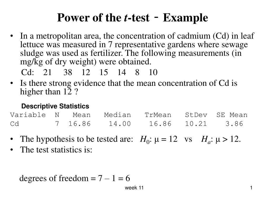
Power of the t -test - Example. In a metropolitan area, the concentration of cadmium (Cd) in leaf lettuce was measured in 7 representative gardens where sewage sludge was used as fertilizer. The following measurements (in mg/kg of dry weight) were obtained.

E N D
Power of the t-test - Example • In a metropolitan area, the concentration of cadmium (Cd) in leaf lettuce was measured in 7 representative gardens where sewage sludge was used as fertilizer. The following measurements (in mg/kg of dry weight) were obtained. Cd: 21 38 12 15 14 8 10 • Is there strong evidence that the mean concentration of Cd is higher than 12 ? Descriptive Statistics Variable N Mean Median TrMean StDev SE Mean Cd 7 16.86 14.00 16.86 10.21 3.86 • The hypothesis to be tested are: H0: μ = 12 vs Ha: μ > 12. • The test statistics is: degrees of freedom = 7 – 1 = 6 week 11
Since t = 1.26 < 1.943, we cannot reject H0 at the 5% level and so there are no strong evidence. The P-value is 0.1 < P(T(6) ≥ 1.26) < 0.15 and so is greater then 0.05 indicating a non significant result. • Find the power of the test when true mean is 13. We can use MINITAB to calculate the power for t-tests. MINITAB commands: Stat > Power and Sample size > 1 sample t 1-Sample t Test Testing mean = null (versus > null) Calculating power for mean = null + 1 Alpha = 0.05 Sigma = 10.21 Sample Size Power 7 0.0788 week 11
What is the probability of a type II error when = 13? • Find the power of the test when true mean is 20. Testing mean = null (versus > null) Calculating power for mean = null + 8 Alpha = 0.05 Sigma = 10.21 Sample Size Power 7 0.5749 • Use the tables to find the power when = 20. • Find the sample size if we specified a desired power of 0.90, when the true mean is 20. 1-Sample t Test Testing mean = null (versus > null) Calculating power for mean = null + 8 Alpha = 0.05 Sigma = 10.21 Sample Size Target Power Actual Power 16 0.9000 0.9104 week 11
Match Pairs t-test • In a matched pairs study, subjects are matched in pairs and the outcomes are compared within each matched pair. The experimenter can toss a coin to assign two treatment to the two subjects in each pair. Matched pairs are also common when randomization is not possible. One situation calling for match pairs is when observations are taken on the same subjects, under different conditions. • A match pairs analysis is needed when there are two measurements or observations on each individual and we want to examine the difference. • For each individual (pair), we find the difference d between the measurements from that pair. Then we treat the dias one sample and use the one sample t – statistic to test for no difference between the treatments effect. • Example: similar to exercise 7.41 on p482 in IPS. week 11
Data Display Row Student Pretest Posttest improvement 1 1 30 29 -1 2 2 28 30 2 3 3 31 32 1 4 4 26 30 4 5 5 20 16 -4 6 6 30 25 -5 7 7 34 31 -3 8 8 15 18 3 9 9 28 33 5 10 10 20 25 5 11 11 30 32 2 12 12 29 28 -1 13 13 31 34 3 14 14 29 32 3 15 15 34 32 -2 16 16 20 27 7 17 17 26 28 2 18 18 25 29 4 19 19 31 32 1 20 20 29 32 3 week 11
One sample t-test for the improvement T-Test of the Mean Test of mu = 0.000 vs mu > 0.000 Variable N Mean StDev SE Mean T P improvem 20 1.450 3.203 0.716 2.02 0.029 • MINITAB commands for the paired t-test Stat > Basic Statistics > Paired t Paired T-Test and Confidence Interval Paired T for Posttest – Pretest N Mean StDev SE Mean Posttest 20 28.75 4.74 1.06 Pretest 20 27.30 5.04 1.13 Difference 20 1.450 3.203 0.716 95% CI for mean difference: (-0.049, 2.949) T-Test of mean difference=0 (vs > 0): T-Value = 2.02 P-Value = 0.029 week 11
Character Stem-and-Leaf Display Stem-and-leaf of improvement N = 20 Leaf Unit = 1.0 2 -0 54 4 -0 32 6 -0 11 8 0 11 (7) 0 2223333 5 0 4455 1 0 7 week 11
Inference for non-normal populations • Three general strategies are available for making inference about the mean of a clearly non-normal distribution based on small sample. • In some cases a distribution other than a normal distribution will describe the data well. There are many non-normal models for data, and inference procedures for these models are available. • Because skewness is the chief barrier to the use of t procedures on data without outliers, we can attempt to transform skewed data so that the distribution is symmetric and as close to normal as possible. CI and P-values from the t procedures applied to the transformed data will be quite accurate for even moderate sample size. • The third strategy is to use a distribution-free inference procedure. Such procedures do not assume that the population distribution has any specific form, such as normal. Distribution-free procedures are often called nonparametric procedures. week 11
The sign test for matched pairs • One way of analyzing nonnormal data is to use a distribution-free procedure, or nonparametric procedure. • Distribution-free (nonparametric) tests have two drawbacks; • They are generally less powerful than the test designed for use with a specific distribution such as t-test. • We must often modify the statement of the hypothesis in order to use the distribution free test. • The simplest distribution free test, and one of the most useful, is the sign test. • Example Use a sign test to test whether attending the Institute improves listening skills (In Exercise 7.41 above). week 11
Solution Step-1: Calculate the differences (post-pre). Ignore pairs with difference 0. Step-2: Count the number of positive differences (X). In our example X=14. The test statistic of the sign test, is the count X of pairs with positive differences. Under the null hypothesis X ~ Bin (20, ½). P-values for X are based on this distribution. Step-3: Test the hypothesis: H0: p = 0.5 vs Ha: p > 0.5 where p is the probability of a positive difference. • Note that this is a test of H0: population median = 0 vs Ha: population median > 0. week 11
The P-value for this test is given by P(X ≥14) = 0.0370+0.0148+0.0046+0.0011+0.0002=0.0577 • MINITAB commands for the sign test Stat > Nonparametrics > 1 sample sign • The MINITAB output for the above problem is given below. Sign Test for Median Sign test of median = 0.00000 versus > 0.00000 N Below Equal Above P Median Diff. 20 6 0 14 0.0577 2.000 week 11
Two-sample problems • The goal of inference is to compare the response in two groups. • Each group is considered to be a sample form a distinct population. • The responses in each group are independent of those in the other group. • A two-sample problem can arise form a randomized comparative experiment or comparing random samples separately selected from two populations. • Example: A medical researcher is interested in the effect of added calcium in our diet on blood pressure. She conducted a randomized comparative experiment in which one group of subjects receive a calcium supplement and a control group gets a placebo. week 11
Comparing two means (with two independent samples) • Here we will look at the problem of comparing two population means when the population variances are known or the sample sizes are large. Suppose that a SRS of size n1 is drawn from an N( μ1, σ1) population and that an independent SRS of size n2 is drown from an N( μ2, σ2) population. Then the two-samplezstatistics for testing the null hypothesis H0: μ1 = μ2 is given by and has the standard normal N(0,1) sampling distribution. • Using the standard normal tables, the P-value for the test of H0 against Ha : μ1 > μ2is P( Z ≥ z) Ha : μ1 < μ2is P( Z ≤ z ) Ha : μ1 ≠ μ2is 2·P(Z ≥ |z|) week 11
Example • A regional IRS auditor runs a test on a sample of returns filed by March 15 to determine whether the average return this year is larger than last year. The sample data are shown here for a random sample of returns from each year. • Assume that the std. deviation of returns is known to be about 100 for both years. Test whether the average return is larger this year than last year. week 11
Solution week 11
Comparing two population means (unknown std. deviations) • Suppose that a SRS of size n1 is drawn from a normal population with unknown mean 1 and that an independent SRS of size n2 is drawn from another normal population with unknown mean 2. To test the null hypothesis H0: 1 = 2, we compute the two sample t-statistic • This statistic has a t-distribution with df approximately equal to smaller of n1 – 1 and n2 - 1. We can use this distribution to compute the P-value. week 11
Example • The weight gains for n1 = n2 = 8 rats tested on diets 1 and 2 are summarized here. Test whether diet 2 has greater mean weight gain. Use the 5% significant level. • The hypotheses to be tested are: H0: μ1 = μ2 vs Ha: μ1 < μ2 . • The test statistic is week 11
The P-value is P(T(7) ≤- 3.65) = P(T(7) ≥ 3.65) , from table D we have 0.005 < P-value < 0.01 and so we reject H0 and conclude that the mean weight gain from diet 2 is significantly greater than that from diet 1 (at the 5% and 1% significant level). • A C% CI for the difference between the two means is given by, • For this example the 95% CI is week 11
The pooled two sample t-procedures • If the two normal population distributions have the same std deviation, i.e. σ1= σ2 = , then we can estimate the common stdev. by, • This is called the pooled estimator of σ2, it combines the information in both samples. • The pooled two-sample t statistic is then, and has exactly a t-distribution with df = n1 + n2 – 2 . week 11
Example • In a study of heart surgery, one issue was the effects of drugs called beta blockers on the pulse rate of patients during surgery. The available subjects were divided into two groups of 30 patients each. The pulse rate of each patient at a critical point during the operation was recorded. The treatment group had mean 65.2 and std dev. 7.8. For the control group the mean was 70.3 and the std dev. was 8.3. a) Do beta-blocker reduce the pulse rate? b) Give a 99% CI for the difference in mean pulse rates. • Denoting the control group as 1 and the treatment group as 2 the solution is … week 11
a) The hypotheses to be tested are: H0: μ1 = μ2 vs Ha: μ1 > μ2 . The pooled standard deviation is and the test statistic is The P-value is P(T(58) ≥ 2.45), using table D and df = 60 we get 0.005 < P-value < 0.01 and so we have significant evidence that the mean pulse rate of the control group is higher than the mean of the treatment group at the 5% and 1% significant level. Does it mean that beta-blocker reduce the pulse rate?! week 11
b) A C level CI’s for μ1 – μ2 is given by For this example, a 99% CI is , = (-0.429 , 10.629 ) • MINITAB command: Stat > Basic Statistics > 2 Sample t . week 11
Example • A study compared various characteristics of 68 healthy and 33 failed firms. One of the variables was the ratio of current assets to current liabilities. Row Firms(Healthy/Failed) Ratio 1 h 1.50 2 h 0.10 3 h 1.76 ... 99 f 0.13 100 f 0.88 101 f 0.09 week 11
Stem-and-leaf of Ratio failed N = 33 Leaf Unit = 0.10 5 0 00111 7 0 22 11 0 4455 12 0 6 (10) 0 8888899999 11 1 111111 5 1 33 3 1 4 2 1 6 1 1 1 2 0 week 11
Stem-and-leaf of Ratio healthy N = 68 Leaf Unit = 0.10 1 0 1 2 0 2 2 0 4 0 66 10 0 899999 15 1 00011 19 1 2223 26 1 4445555 34 1 66666777 34 1 88888889999 23 2 0000111 16 2 222223 10 2 455 7 2 6677 3 2 8 2 3 01 week 11
Two Sample T-Test and Confidence Interval Two sample T for Ratio Firms N Mean StDev SE Mean failed 33 0.824 0.481 0.084 healthy 68 1.726 0.639 0.078 95% CI for mu (f) - mu (h): ( -1.129, -0.675) T-Test mu (f) = mu (h) (vs <): T = -7.90 P = 0.0000 DF = 81 Two Sample T-Test and Confidence Interval (pooled test and CI) Two sample T for Ratio Firms(He N Mean StDev SE Mean f 33 0.824 0.481 0.084 h 68 1.726 0.639 0.078 95% CI for mu (f) - mu (h): ( -1.151, -0.652) T-Test mu (f) = mu (h) (vs <): T = -7.17 P = 0.0000 DF = 99 Both use Pooled StDev = 0.593 week 11