LECTURE 4 - Seismology Hrvoje Tkalčić

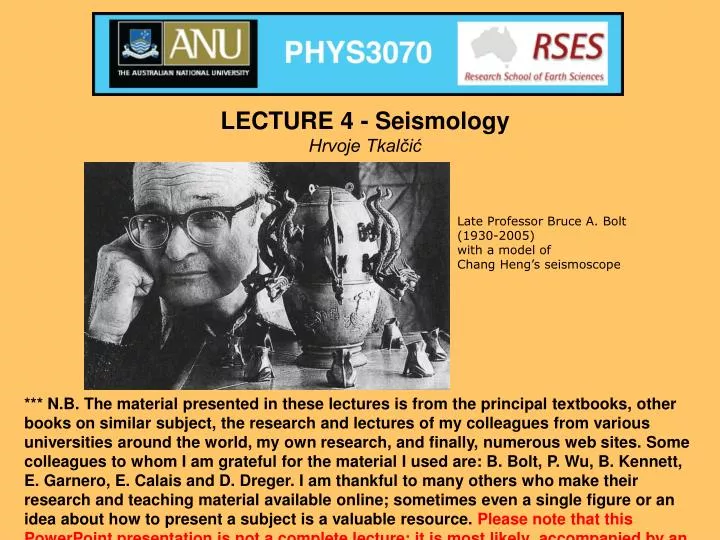
1. LECTURE 4 - Seismology Hrvoje Tkalčić Late Professor Bruce A. Bolt (1930-2005) with a model of Chang Heng’s seismoscope *** N.B. The material presented in these lectures is from the principal textbooks, other books on similar subject, the research and lectures of my colleagues from various universities around the world, my own research, and finally, numerous web sites. Some colleagues to whom I am grateful for the material I used are: B. Bolt, P. Wu, B. Kennett, E. Garnero, E. Calais and D. Dreger. I am thankful to many others who make their research and teaching material available online; sometimes even a single figure or an idea about how to present a subject is a valuable resource. Please note that this PowerPoint presentation is not a complete lecture; it is most likely accompanied by an in-class presentation of main mathematical concepts (on transparencies or blackboard).***

2. Earthquakes as natural disasters: can we predict them? San Francisco, 1906 Tokyo-Yokohama, 1923 • Victims in Banda Aceh, Indonesia, after the Sumatra-Andaman earthquake and tsunami in 2004 Pakistan, 2005

3. Strong motion simulation in SF Bay Area A simulation of the San Simeon earthquake, CA, through a model of 3D structure. This is achieved using a numerical finite difference method on a grid of points. The main wave front is visibly refracted or bent by contrasts in the velocity across both the Hayward and San Andreas faults. Concentrations of high amplitude standing waves persist throughout the movie around San Jose and in San Pablo Bay. These areas are low-velocity sedimentary basins and cause the amplitudes of ground motion to be amplified as well as extend the duration of the motions. Both of these factors increase the level of hazard to structures. Berkeley Oakland San Andreas Hayward San Francisco San Jose A simulation movie Courtesy of Prof. Douglas Dreger, UC Berkeley and Dr. Shawn Larsen, LLNL

4. Seismology as a tool for probing the internal structure of the Earth

5. Global shear velocity structure Lithospheric structure under Australia Li and Romanowicz 1996 van der Hilst, Kennett and Shibutani 1998 Some examples of seismic tomography Compressional velocity structure in the lowermost mantle Tkalčić, Romanowicz and Houy 2002

6. The beginnings An artist’s conception of the Chinese scholar Chang Heng contemplating his seismoscope. Balls were held in the dragons’ mouth by lever devices connected to an internal pendulum. The direction of the first main impulse of the ground shaking was reputed to be detected by the particular ball that was released.

7. Early seismographs and advances in seismology • John Milne - constructed the first reliable • seismograph in 1892 • F. Reid - elastic rebound model in 1906 after the • Great San Francisco Earthquake and fire • Earthquakes happen on preexisting faults • A notion that the core is needed to explain seismic • travel time proposed by R, Oldham in 1906 Emil Wiechert (1861-1928) The 1200 kg Wiechert seismograph for measuring horizontal displacements

8. Probing the Earth with seismology: European discoverers of seismic discontinuities Andrija Mohorovičić (1857-1936) Crust-Mantle boundary 1910 Beno Gutenberg (1889-1960) Mantle-Core boundary 1914 Inge Lehmann (1888-1993) Inner Core 1936 Recipe for longevity: study the inner core!

9. The Earth’s Interior CRUST-MANTLE BOUNDARY Mohorovičićdiscontinuity (Moho) (1910) CORE-MANTLE BOUNDARY Discovered by B. Gutenberg (1914) INNER CORE Discovered by I. Lehmann (1936) * For Comparison: Pluto discovered in 1931

10. Berkeley Seismographic Station • The first seismographs in the western hemisphere • installed at the University of California Berkeley campus • in 1887 (largely due to the interest of astronomers). • The occurrence of the San Francisco Great Earthquake and Fire in 1906 began a new era in seismology. The east-west component of ground motion at the Berkeley station recorded by the Bosch Omori seismograph on March 10, 1922, from an earthquake source near Parkfield, California. The recording is part of the basis of the "Parkfield Prediction Experiment" (1988 ± 5 years). Reproduced on a wine label printed for the Centennial Symposium, May 28–30, 1987. Portion o seismograms recorded by the short-period vertical-component
seismographattheJamestownstationoftheUniversity of California Berkeleynetwork.
ThewavepacketAisthecorephaseP4KP, andBisP7KP. These exotic seismic phases are multiple reflections from the lower side of the core mantle boundary.

11. Seismographs on the Moon APOLLO 11 Astronaut Edwin E. Aldrin Jr., lunar module pilot, is photographed during the Apollo 11 extravehicular activity on the Moon. He has just deployed the Early Apollo Scientific Experiments Package (EASEP). In the foreground is the Passive Seismic Experiment Package (PSEP); beyond it is the Laser Ranging RetroReflector (LR-3); in the left background is the black and white lunar surface television camera; in the far right background is the Lunar Module. Astronaut Neil A. Armstrong, commander, took this photograph with a 70mm lunar surface camera. APOLLO 14 Astronaut Alan B. Shepard Jr., foreground, Apollo 14 commander, walks toward the Modularized Equipment Transporter (MET), out of view at right, during the first Apollo 14 extravehicular activity (EVA-1). An EVA checklist is attached to Shepard's left wrist. Astronaut Edgar D. Mitchell, lunar module pilot, is in the background working at a subpackage of the Apollo Lunar Surface Experiments Package (ALSEP). The cylindrical keg-like object directly under Mitchell's extended left hand is the Passive Seismic Experiment (PSE).

12. Hooke’s Law of elasticity • When a force is applied to a material, it deforms: stress induces strain • – Stress = force per unit area • – Strain = change in dimension • For some materials, displacement is reversible = elastic materials • – Experiments show that displacement is: • Proportional to the force and dimension of the solid • Inversely proportional to the cross-section • – One can write: ΔL ∝ FL/A • – Or ΔL/L ∝ F/A • –Strain is proportional to stress = Hooke’s law • – Hooke’s law: good approximation for many Earth’s materials when ΔL is small 1660 Robert Hooke

13. Stress and strain • Stress-strain relation: • Elastic domain • Stress-strain relation is linear • Hooke’s law applies • Beyond elastic domain • Initial shape not recovered when stress is removed • Plastic deformation • Eventually stress > strength of material => failure • Failure can occur within the elastic domain = brittle behavior • Strain as a function of time under stress • Elastic = no permanent strain • Plastic = permanent strain • What is the mathematical relation between stress and strain?

14. Normal strain x1 The series expansion of u1:

15. Shear strain Stress and strain x2 For small deformations: The series expansion of u2: and since u2(A)=0: x1 Similarly, for AD segment:

16. Shear tensor

17. Dilatation For products of u, v, w ≈ 0

18. Stress Stress and strain Internal traction (stress): The stress field is the distribution of internal "tractions" that balance a given set of external tractions and body forces. ij = Stress tensor: ij Direction of the stress component Normal to the surface upon which the stress acts xx = 11, xy= 12etc. using the notation we used for strain

19. A cubic element in static equilibrium For a medium to be in stable equilibrium, the moments must sum to zero. Moments are given by the product of a force times the perpendicular distance from the force to a reference point. Let’s consider a moment around x3 axis first: As x1, x2 -> 0, we have 12= 21 Similarly, for the moments around x1 and x2 axes, 13= 31 and 23= 32. Thus, stress tensor is also symmetric, with 6 independent elements.

20. The most general form of Hooke’s law The constants of proportionality, Cijkl are elastic moduli. We saw that the both strain and stress tensors are second-order tensors, which are symmetric and have 6 independent elements. Cijkl is thus a third-order tensor and in its most general form consists of 81 elements. However, since the strain and stress tensors only have 6 independent elements, the number of independent elements in Cijkl can be reduced to 36. The first stress element is related to the strain elements by: For an isotropic medium (material properties independent on direction or orientation of sample), the number of elastic moduli can conveniently be reduced to only 2. These elastic moduli are called the Lamé constants and . where ij is Krönecker delta function (ij=0 when ij and ij=1 when i=j). This was formulated by Navier in 1821 and Cauchy in 1823.

21. Definitions of elastic moduli - from Lay and Wallace book