Download
1 / 19
200 likes | 353 Views
Section 6.5: Partial Fractions and Logistic Growth. These are called non-repeating linear factors. 1. This would be a lot easier if we could re-write it as two separate terms. You may already know a short-cut for this type of problem. We will get to that in a few minutes. 1.

E N D
These are called non-repeating linear factors. 1 This would be a lot easier if we could re-write it as two separate terms. You may already know a short-cut for this type of problem. We will get to that in a few minutes.
1 This would be a lot easier if we could re-write it as two separate terms. Multiply by the common denominator. Set like-terms equal to each other. Solve two equations with two unknowns.
1 This technique is called Partial Fractions Solve two equations with two unknowns.
1 The short-cut for this type of problem is called the Heaviside Method, after English engineer Oliver Heaviside. Multiply by the common denominator. Let x= - 1 Let x= 3
1 The short-cut for this type of problem is called the Heaviside Method, after English engineer Oliver Heaviside.
2 If the degree of the numerator is higher than the degree of the denominator, use long division first. (from example one)
We have used the exponential growth equation to represent population growth. The exponential growth equation occurs when the rate of growth is proportional to the amount present. If we use P to represent the population, the differential equation becomes: The constant k is called the relative growth rate.
The population growth model becomes: However, real-life populations do not increase forever. There is some limiting factor such as food, living space or waste disposal. There is a maximum population, or carrying capacity, M. A more realistic model is the logistic growth model where growth rate is proportional to both the amount present (P) and the carrying capacity that remains: (M-P)
Logistics Differential Equation The equation then becomes: We can solve this differential equation to find the logistics growth model.
Partial Fractions Logistics Differential Equation
Logistics Growth Model Notes: 1.) A population is growing the fastest when it is half the carrying capacity. 2.) The population will approach its carrying capacity in the long run. (t = ∞)
Example: Logistic Growth Model Ten grizzly bears were introduced to a national park 10 years ago. There are 23 bears in the park at the present time. The park can support a maximum of 100 bears. Assuming a logistic growth model, when will the bear population reach 50? 75? 100?
Ten grizzly bears were introduced to a national park 10 years ago. There are 23 bears in the park at the present time. The park can support a maximum of 100 bears. Assuming a logistic growth model, when will the bear population reach 50? 75? 100?
Bears Years We can graph this equation and use “trace” to find the solutions. y=50 at 22 years y=75 at 33 years y=100 at 75 years