Interpretation of Seafloor Gravity Anomalies

1. Interpretation of Seafloor Gravity Anomalies

2. Gravity measurements of the seafloor provide information about subsurface features. • For example they help resolve : • -the structures that exist at the boundary between oceans and continents • - the dimensions of mid-ocean ridge magma chambers • - the presence and dimensions of offshore sedimentary basins • Gravity surveys of continents reveal additional information about the processes that lead to the rifting of continents and the formation of ocean basins.

3. A gravity anomaly is the difference between the measured value and an expected value. Gravity Anomalies Are calculated: g = gmeasured +/- correction - ggeoid = gravity anomaly gmeasured may be corrected for: •Bouguer •Free Air •Topography and others Whenever a measured value departs from an expected value, an anomaly exists. Corrections are applied to the measured value, depending on one’s interest.

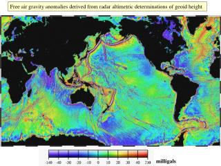
4. Free Air (=Elevation) Corrections gm Mountain Geoid Ocean go The free-air correction accounts for the difference in elevation between the gravimeter and the geoid. For measurements at sea, this is really small! Recall that the difference between sea level and the geoid is slight. go = gmeasured (1 + 0.00031 h) g in gal, height in meters

5. Free Air (=Elevation) Corrections gm Mountain Geoid Ocean go Most free-air gravity anomalies are in the range of a few hundred milligal, while most shipboard corrections are close to one milligal. If the gravimeter is below sea level, the correction must be subtracted. go = gmeasured (1 + 0.00031 h) g in gal, height in meters

6. Bouguer (=Mass) Corrections gh Mountain Geoid Ocean go The Bouguer correction accounts for the additional gravitational attraction between the material that lies between the gravimeter and the geoid.

7. Bouguer (=Mass) Corrections gh Mountain Geoid Ocean go The meaning of the term “free-air correction” becomes more apparent in relation to the Bouguer correction. The free-air correction assumes only air lies between the gravimeter and the geoid; the Bouguer correction assumes material other than air lies between them...

8. Bouguer (=Mass) Corrections One assumes for the Bouguer correction that the mass between the gravimeter and the geoid is that of an infinite plate of uniform density and thickness. The Bouguer correction on land is in the opposite direction of the free-air correction; the added attraction of the extra mass increases the observed gravity. gm Mountain Geoid Ocean go go = gmeasured (1 - 0.00004 h•density) g in gal, height in meters, density in g cm-3

9. Bouguer (=Mass) Corrections To apply a Bouguer correction to gravity measurements, the composition and density of the slab must be known, or inferred. Terrestrial data that are corrected for both elevation and mass (i.e., free air and Bouguer corrections) should approach the same value of g (gravitational attraction) as that of the geoid, provided the local relief is not great. gm Mountain Geoid Ocean go go = gmeasured (1 - 0.00004 h•density) g in gal, height in meters, density in g cm-3

10. Bouguer (=Mass) Corrections at Sea The Bouguer correction at sea substitutes for seawater a layer with the same density as the seafloor. This removes the effects of variations in bottom topography from the gravity data, and makes the data useful for studies of the subsurface. This correction is often made in nearshore gravity surveys that extend onto land. gh Mountain z Geoid Ocean go gcorr = gmeas [1 + 2Gz(dseafloor-dseawater)] g in mgal, height in meters, density in g cm3

11. Topographic Corrections Topography also affects gravity. A gravimeter next to a mountain is attracted to the mountain. The outward directed (upward) component of the attraction decreases the gravitational attraction experienced by its mass. gh Mountain Geoid Ocean go For land areas with large variations in topography, this correction is important. Examples: Pikes Peak, CO 48 mgal Mt. Blanc, France 123 mgal

12. Topographic Corrections For data collected at sea, this type of correction is incorporated in what is known as a 3-dimensional Bouguer correction. It differs from a simple Bouguer correction in that the gravitational attraction of nearby seafloor is also considered. gh Mountain Geoid Ocean go Examples: Pikes Peak, CO 48 mgal Mt. Blanc, France 123 mgal

13. Free-Air Anomaly Over a Subduction Zone +200 Central Aleutian Trench 0 -200 0 The large positive anomaly (more than expected gravitational attraction) above the island arc represents a mass excess (the descending slab). The large negative anomaly (less than expected gravitational attraction) above the trench represents a mass deficiency (low density overlying sediments and the trench itself). Kilometers 300

14. Free-Air Anomaly Over a Subduction Zone +200 Central Aleutian Trench 0 -200 0 The free air gravity anomaly is near zero away from the plate boundary. This indicates the oceanic crust is in isostatic equilibrium. Isostacy= Mass excesses at the Earth’s surface are balanced by mass deficiencies, below the surface. Kilometers 300

15. Japan Plate Free-Air Gravity Anomalies Japan Pacific Plate Triple Junction Philippine Plate Japan Trench

16. Free Air Anomaly For Atlantic Continental Margin Upper Continental Crust Oceanic Crust Upper Mantle Rift Stage Crust The large positive anomaly near the shelf edge (more than predicted gravity) occurs because high density basalts lie underneath the shelf. This high density “basement” rock formed during the initial stages of rifting between North America and Africa. The large negative anomaly seaward of the shelf edge is evidence of a large volume of accumulated sediment. Lower Continental Crust Coastline

17. Free Air Anomaly For Atlantic Continental Margin Upper Continental Crust Oceanic Crust Upper Mantle Rift Stage Crust Lower Continental Crust The location of the boundaries between continental and ocean crust are poorly known. Subsurface geology such as that above is a “best fit” solution to gravity and seismic surveys. Coastline Only for a few continental margin locations, interpretations have been drawn from drilling data.

18. The decrease in the gravity anomaly along the transect suggests a large mass of low density material beneath the ridge crest. The shape of the magma chamber (seen in cross section) is estimated from the gravity data. Bouguer Anomaly Mid-Ocean Ridge (Magma Chamber)

19. From: J. R. Ridgway, M.A. Zumberge, and J.A. Hildebrandat Scripps Institute of Oceanography Source: http://spot.ucsd.edu/towdog/towdog.html The resolution of small, subsurface seafloor features in gravity data improves as the gravitometer is towed closer to the features. Sour From Submersible gravitometer system named Tow Dog

20. Three Tow Dog transects over ~10 km of seafloor. This information, along with ship’s speed data, is needed to correct for gravity variations resulting from Tow Dog’s depth in the water column and vertical acceleration.

21. Free-air gravity tracks above provide very high resolution information about the dimensions of a small offshore sedimentary basin. Many layers of low density sediments in the basin result in lower gravity anomalies over the basin’s center. Gravity (mgal) Distance (km)

22. The image above shows the Bouguer anomaly map for the continental US. The effect of topography and elevation removedby theBouguer correction. The reds are positive anomalies (higher than expected gravity) and the blues are negative anomalies (lower than expected gravity). Many of the red areas are the result of ancient rift systems that contain denser basalts.

23. The image above shows the Bouguer anomaly map for the continental US. The effect of topography and elevation removedby theBouguer correction. The reds are positive anomalies (higher than expected gravity) and the blues are negative anomalies (lower than expected gravity). Many of the red areas are the result of ancient rift systems that contain denser basalts.

24. Red along the Atlantic and Gulf coast margins results from subsurface basalt formed during the break-up of Pangea and the birth of the Atlantic ocean. The blue areas of the Rockies and Sierra suggest that these mountains are in isostatic equilibrium, meaning that they have deep, low-density granitic “roots”.

25. gm Mountain Geoid Ocean go Evidence of Isostacy • Free Air GravityAnomalies for most of Earth’s surface are close to zero There must be an equilibrium state ... ISOSTACY Implies that the mass excesses at surface are balanced by mass deficits at depth.

26. In this model, mountains have deep roots. The dashed line is an isostatic level; along this line, the weight of the overlying material is the same. Airy Isostacy Crust 2.7 g /cc Mantle >3.3 g /cc

27. Can you name a major feature of the seafloor that is an example of Pratt isotacy? Pratt Isostacy  Crust          Mantle Another type of balance (model), known as Pratt isostacy. The density of the overlying material varies throughout a topographic feature. The isostatic level here is the boundary between crust and mantle.