Download
1 / 27
270 likes | 276 Views
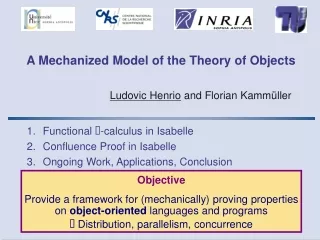
A Locally Nameless Theory of Objects. Ludovic Henrio, Florian Kamm ül ler, Bianca Lutz, and Henry Sudhof. Introduction: -calculus and De Bruijn notation locally nameless technique formalization in Isabelle and proofs. SAFA workshop – Oct 2010. Context.

E N D
A Locally Nameless Theory of Objects Ludovic Henrio, Florian Kammüller, Bianca Lutz, and Henry Sudhof Introduction: -calculus and De Bruijn notation locally nameless technique formalization in Isabelle and proofs SAFA workshop – Oct 2010
Context • Calculi abstract away real programming languages: • Proofs made on the calculus allow optimisation and ensure properties on real programs • Use of theorem prover to increase confidence in those proofs • A general problem is the representation of variables • We focus here on a simple object language
Each method is a function with a parameter: “self” Functional -calculus • Syntax • Semantics (Abadi - Cardelli) • Why functional? updating a field creates a new object (copy)
What are De Bruijn Indices? • De Bruijn indices avoid having to deal with -conversion • equivalent to • Variables are natural numbers depending on the depth of the parameter also represents
Why De Bruijn Indices? Unique representation -> avoids dealing with alpha conversion • Drawbacks: • Terms are “ugly” We are interested ingeneral properties / not for extracting an interpreter … • Definition of subst and lift: semantics more complex • Proofs of many additional (easy) lemmas • Advantages • Established approach • Reuse Nipkow’s framework for confluence of the -calculus • Alternative approaches, e.g. locally nameless
What is locally nameless technique? • Bound variables are represented by their De Bruijn index • Free variables are represented by a “usual” variable manipulate only locally closed terms i.e. all indexed variables must be bound and are forbidden
Opening and Closing • open and close change between bound and free variables • helps maintain the “locally closed” invariant non-LC terms open close
A method parameter • Syntax open close
Cofinite Quantification • When specifying semantics or proving properties, we need to open terms: • x cannot be taken randomly, an idea: • Typically, proofs by induction, we must prove: • Sometimes impossible if t’≠t, similar problem for: • We use cofinite quantification: t’ t x
Semantics with cofinite quantification • Reduce inside update (adapted for self+parameter):
Properties and Proofs • Translated proofs for De Bruijn: • Confluence • Typing: subject reduction and progress • Different lemmas: • lifting and manipulation of indices for De Bruijn • Translation between free and bound variables for LN • Not particularly shorter, but LN more precise • Induction scheme more complex due to more complex semantics (cofinite quantification)
Conclusion on LN representation • New concepts wrt de Bruijn: • opening and closing • locally closed terms (precondition of many lemmas and semantic rules) • cofinite quantification • Better structure, accuracy, and understanding: • Distinction between free and bound variables • Cofinite quantification • LN adapted to objects and to multiple parameters • Terms can be written in a similar manner as paper version (using closing)
Other techniques? • Nominal techniques: • Terms are identified as a set bijective to all terms factorised by alpha-equivalence • There must be a finite support for a term t • Well supported in Isabelle but not adapted to finite maps for the moment • Higher Order Abstract Syntax • binders represented by binders of the meta-level • not very convenient in our case
p r q Diamond confluent: Confluence Principles • Ensures that all computations are equivalent (same result) • Generally based on a diamond property: a b s c d 2 - Confluence
confluent Confluence Principles (2) • In general we have to introduce a new reduction that verifies the diamond property a b c and d 2 - Confluence
Confluence of the -calculus • Based on Nipkow’s framework: Confluence for the -calculus • Useful lemmas: commute, Church-Rosser, diamond • Structure of a confluence proof in Isabelle • Definition of a parallel reduction (verifies diamond) • Like for -calculus, can reduce all sub-terms in parallel • Also includes (semantics of the -calculus) 2 - Confluence
Reducing in Parallel inside Object • Subgoal (looks trivial but proof is tricky): • Solution: split into several reductions on object fields • -calculus confluence proof similar to Nipkow’s framework but: • Much less automatic • Difference of granularity between lists of terms and objects • More cases for diamond (more constructors/rules) Number of methods 2 - Confluence
In the Meantime … • Objects as finite maps from labels to methods instead of lists of methods • Definition of finite maps and a new induction principle • Closer to original -calculus (syntax and semantics); new recurrence principle on terms • Formalization of the basic type system for the functional -calculus • Typing rules (Abadi - Cardelli) • Subject reduction, progress (no stuck configuration) 3 - Ongoing Work, Applications, Conclusion
Todo List • Remove De Bruijn indices “nominal techniques”? • Introduce methods with a parameter: (x,y) / a.l(b) • Apply to other results on object languages (concurrence, mobility, …) • A base model for Aspect Oriented Programming 3 - Ongoing Work, Applications, Conclusion
Towards Distribution • A model for the ASP calculus in Isabelle; ASP formalizes: • Active objects (AO) without shared memory • AO is the entry point and the master object of the activity • Communicating by asynchronous method calls with futures • Currently: • Definition of a functional ASP in Isabelle • Proof of well-formedness of the reduction (no creation of reference to non-existing active objects or futures) • To do …. • A type system for ASP • Proof of confluence for the functional ASP • Extension of the concurrency in the functional calculus • Case of the imperative ASP calculus … 3 - Ongoing Work, Applications, Conclusion
Conclusion • A formalization of the -calculus in Isabelle • A confluence proof for the functional -calculus • Parallel reduction inside objects • A base framework for developments on objects, confluence and concurrency • A lot of possible applications (distribution / typing / AOP …) Experiments on Isabelle (few months development) • User-friendly, relatively fast development • Finding the right structure/representation is crucial • Difficulties when modifying / reusing code http://www.cs.tu-berlin.de/~flokam/isabelle/sigma/ 3 - Ongoing Work, Applications, Conclusion