Download
1 / 27
270 likes | 271 Views
Learn about polynomial curves and their modelling techniques, including Bézier curves. Explore the geometric connections between control points and curves, and discover the de Casteljau algorithm for generating points on the curve. Understand the properties and applications of Bézier curves in various modelling scenarios.

E N D
Polynomial Curves Lecture 5 (Modelling)
Modelling • Modelling Techniques: • Polygon Mesh Models • Spline-based Curves and Surfaces: Bézier, B-spline, NURBS and subdivision curves and surfaces. [2 lectures] • Constructive Methods: boolean set operations, sweeps, surfaces of revolution, generalized cylinders, spatial deformation. [1 lecture] • Volumetric Models: implicit surfaces, voxels, and the marching cubes algorithm. [1 lecture]
Polynomials • An th degree polynomial has the form: • Where are the coefficients and are the power terms. • The degree, , is the highest power to which is raised • The order is the number of coefficients ( ). • Constant: • Linear: • Quadratic: • Cubic:
Polynomial Curves • If the coefficients are 2D or 3D points and is restricted to a range, e.g. , then a polynomial represents a parametric curve. • The coefficients are called control points. • Often represented in basis form: • Where is a point on the curve, are the control points and are the basis functions. • Example:
Bases • Power Basis: • Problem: with a power basis it is very difficult to predict the shape of the curve from the position of the control points. Also it is given to numerical instability. • Solution: use other basis functions (Hermite, Bézier and B-spline).
Bézier Curves • Discovered independently in the early 70’s by Bézier and de Casteljau. Both worked in the automobile industry. • Bézier curves are popular because there is a clear geometric connection between the control points and the curve: • Interpolates the first and last control points: . • The tangent vectors at the endpoints are aligned with the line segments, and . • The curve lies in the convex hull of its control points. Imagine the convex hull as a rubber band allowed to snap tight around the control points.
Bézier (Bernstein) Basis • Binomial coefficient function: • The binomial coefficients can be quickly derived using Pascal’s triangle (terms are summed from above diagonally left and right):
Constant and Linear Bézier Curves • Constant (a point): • Linear (a line segment):
Quadratic and Cubic Bézier Curves • Quadratic: • Cubic:
The de Casteljau Algorithm • A recursive in-betweening (linear interpolation) process which can be used to: • Generate a point on the curve (the alternative is to evaluate the Bézier curve equation). • Split a Bézier curve into two halves. • Working from the initial control polygon (the line segments joining adjacent control points): • a point is placed of the way along each edge. • These points are joined into a new control polygon. • The process is repeated until only a single point is introduced. • This is the point at parameter on the curve.
de Casteljau Specifics • The recurrence relation is: • Where are the original control points and is the point on the curve. • The intermediate control points constitute two Bézier curves split from the original at :
Properties • Endpoint Interpolation: • The Bézier curve passes through (interpolates) the first and last control points. • Affine Invariance: • Instead of transforming potentially many individual points on the curve, the control points are transformed. This is similar to the property that affine transformations preserve straight lines.
More Properties • Convex Hull Property: • The curve never wanders outside the convex hull. This hull is defined as the set of all convex combinations of control points: • Linear Precision: • A high degree Bézier curve can be forced into a straight line segment by placing the control points on a straight line. • Variation Diminishing Property: • Bézier curves cannot ‘wiggle’ more than their control polygon. In 2D, no straight line can intersect the curve more times than it intersects the control polygon.
Exercise I: Circles and Bézier Curves • Explain why it is impossible to approximate a circle with a single closed cubic Bézier curve. • Reminder: means that the tangent vectors at joins are equal. Closed means that the curve starts and ends at the same point. • Find the control point positions for a cubic Bézier curve which approximates (as closely as possible) a semi-circle of radius . • Hint: you will need to use endpoint interpolation, endpoint tangents and evaluation of the curve at to solve this problem.
Solution I: Circles and Bézier Curves • (a) Closed curve (b) continuous at (c) All control points are collinear which implies, by the convex hull property, that . (d) This is a point not a circle.
Solution I: Continued • (a) Endpoints must lie where the circle cuts the -axis: (b) For continuity with the lower semicircle must lie along vertical lines from and at the same height (by symmetry) (c) To find : The semicircle cuts the -axis at . We want to ensure that the Bézier curve passes through this point.
The Problem of Local Control • Bézier curves are geometrically intuitive but they fail to provide local control. • A designer cannot concentrate on altering part of a Bézier curve without affecting the rest. • This is because the basis functions, which define the weight (influence) given to each control point, are all non-zero over . So, each control point has some influence over the shape of the whole curve. • Solution: build a curve by piecing together polynomial segments. • This is the purpose behind B-spline curves.
Chaikin’s Corner Cutting • Take a control polygon and cut each edge at the and marks. • Join these new points across the corners to create a refined (subdivided) control polygon. • This process can be repeated, producing a successively smoother curve. • In the limit, a quadratic B-spline curve results. • Note: each control point only influences a local portion of the curve.
B-splines • B-spline curves are piecewise polynomials which consist of one or more segments. • The point at which segments meet (usually with continuity) are called joints. • Each segment has an associated parameter interval – a span. • A joint occurs at a particular parameter interval – a knot. • The B-spline basis functions associated with a control point is non-zero over a limited number of spans (at most ). This achieves local control.
Cox-de Boor Recurrence • B-spline basis functions are built recursively from two lower degree B-splines. • Given: the number of spans , degree , control points , knot vector and curve domain . • The B-spline curve equation is: • Cox-de Boor recurrence defines the B-spline basis fns:
Examples of Cox-de Boor Recurrence • Examples:
Effects of the Knot Vector • Initial Curve
Narrowing a Span • Narrowing a Span • Effect: One interval is compressed and another expanded. The curve stretches closer to one of the control points.
Duplicating Knots • Multiple Knots • Effect: The continuity of the basis fns. and matching curve is decreased. If a knot has multiplicity then one of the control points is interpolated.
Standard Knot Vectors • Uniform • All knots are evenly spaced, usually by a unit interval, e.g. . This means that all the basis functions have the same shape and are just translated versions of a single function. Full Cox-de Boor recurrence is not needed. • Open Uniform • Equally spaced knots, but the end points have multiplicity , e.g. . Such a curve interpolates the endpoints and can have multiple segments.
B-spline Properties • Continuity: • At a particular joint , a B-spline curve exhibits continuity, where is the curve degree and is the multiplicity of the knot at . • Local Control: • B-spline basis functions have compact support. They are non-zero over a limited number of spans (in fact B-splines are defined to have minimal support). Compact support implies that control points affect a limited number of segments. • Affine Invariance: • To transform a B-spline curve, simply transform the control points and generate the new curve.
More B-spline Properties • Strong Convex Hull Property: • A B-spline curve segment lies in the convex hull of the active (non-zero weighted) control points influencing that segment. This provides a tighter hull than the convex hull of the entire curve. • Linear Precision: • If control points are collinear then the corresponding segment is a straight line. • Variation Diminishing: • A given plane will not intersect a B-spline curve more often than it intersects the control polygon. • B-spline Curves include Bézier Curves: • A Bézier curve is a B-spline curve with the knot sequence where superscript denotes knot multiplicity.