Download
1 / 16
160 likes | 179 Views
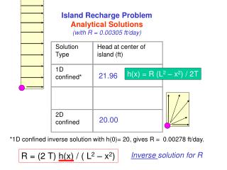
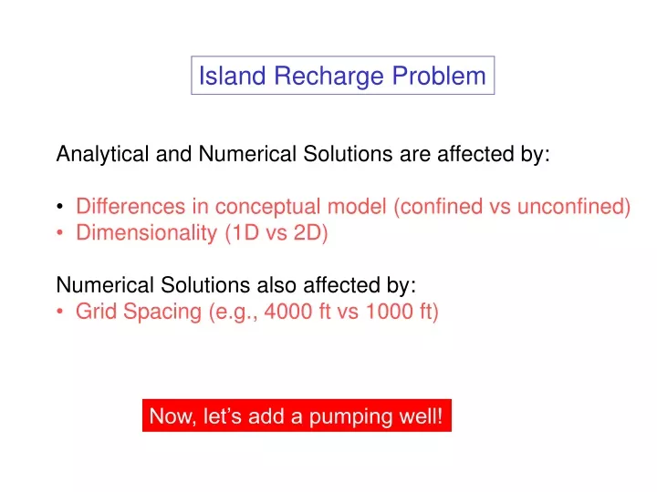
Island Recharge Problem. Analytical and Numerical Solutions are affected by: Differences in conceptual model (confined vs unconfined) Dimensionality (1D vs 2D) Numerical Solutions also affected by: Grid Spacing (e.g., 4000 ft vs 1000 ft). Now, let’s add a pumping well!. Q. R x y.

E N D
Island Recharge Problem • Analytical and Numerical Solutions are affected by: • Differences in conceptual model (confined vs unconfined) • Dimensionality (1D vs 2D) • Numerical Solutions also affected by: • Grid Spacing (e.g., 4000 ft vs 1000 ft) Now, let’s add a pumping well!
Q R x y y x Point source (L3/T) Distributed source (L3/T) R = Q/x y
P = - R Distributed sink In a finite difference model, all sinks (including pumping) are represented as distributed sinks.
Island Recharge Problem ocean L y 2L well ocean ocean Only ¼ of the pumping well is in the upper right hand quadrant. Qwell = QT / 4 x ocean
Bottom 4 rows Assume pumping from the well where: Qwell = 0.1 IN & IN is the inflow to the top right hand quadrant. Pumping is treated as a diffuse sink. Well P = Qwell / {(x y)/4} = Qwell / (a2/4) = 4 Qwell / a2
Also: where: QT = 0.1 [ (4)(IN) ] IN is the inflow to the upper right hand quadrant.
Write a new finite difference expression P = 0 except at the pumping well where P = 4Qwell/a2
Bottom 4 rows Pumping is treated as a diffuse sink. Well Head computed by the FD model is the average head in the cell, not the head in the well.
Q P x y y x Point sink (L3/T) Distributed sink (L3/T) P = Q/x y Finite difference models simulate all sources/sinks as distributed sources/sinks; finite element models simulate all sources/sinks as point sources/sinks.
Use eqn. 5.1 (Thiem equation for confined aquifers) or equation 5.7 (unconfined version of the Thiem equation) in A&W to calculate an approximate value for the head in the pumping well in a finite difference model.
unconfined aquifer confined aquifer Thiem equation for steady state flow to a pumping well. Figure from Hornberger et al. 1998
Use eqn. 5.1 (confined aquifer) or 5.7 (unconfined aquifer) in A&W to calculate an approximate value for the head in the pumping well in a finite difference model. Sink node (i, j) r = a re (i+1, j) hi,j is the average head in the cell. reis the radial distance from the node where head is equal to the average head in the cell, hi,j Using the Thiem eqn., we find that re = 0.208 a
Solution by Iteration • Gauss-Seidel Iteration • SOR (Successive Over Relaxation)
In SOR (successive over-relaxation): SOR relaxation factor G-S where c = error or residual
SOR Formula Relaxation factor = 1 Gauss-Seidel < 1 under-relaxation >1 over-relaxation where, for example, (Gauss-Seidel Formula for Laplace Equation)
SOR solution for confined Island Recharge Problem The Gauss-Seidel formula for the confined Poisson equation where Spreadsheet