Servo Tuning Tutorial

1. Servo Tuning Tutorial

2. Presentation Outline • Introduction • Servo system defined • Why does a servo system need to be tuned • Trajectory generator and velocity profiles • The PID Filter • Proportional gain • Derivative Gain • Integral Gain • Tuning a servo • Servo Tuning program controls • Initial settings • The first move • Setting the proportional gain • Setting the derivative gain • Setting the integral gain • Saving the PID and trajectory parameters • Analyzing the performance of the servo

3. Introduction Almost everyone who has worked with servo systems has had at least one challenging experience while trying to tune a servo. Theory often doesn’t seem to work very well in practice. And oftentimes successfully tuning a servo requires a lot of trial and error. In this tutorial we will try to remove some of the mystery and help you reduce the amount of trial and error required to succeed. #1 – First, what is a Servo? The dictionary describes a servomechanism as: An automatic system in which the output is constantly compared with the input through some form of feedback. The error (or difference) between the two quantities can be used to bring about the desired amount of control. But this is a generic definition which doesn’t really tell us very much.

4. We will more specifically define this automatic system as a closed loop servo system which is comprised of: • An electric motor, typically DC brush or DC brushless • A servo amplifier, which provides drive current to the motor • A motor feedback device, typically an incremental quadrature encoder • A motion controller Motion Controller Typical closed loop servo system

5. #2 – Why does a servo need to be tuned? Upon receiving a motion command from the user, if the servo system has not been tuned the servo controller cannot calculate the appropriate torque/velocity command to apply to the servo amplifier. Imagine a seesaw, with the +/- 10 volt torque/velocity command on one side and the response of the motor/load (feedback from an encoder) on the other side. Until the servo is tuned, the system is effectively out of balance. Only after a servo has been tuned can the controller calculate the appropriate torque/velocity command output for a given user defined motion. The behavior of an improperly tuned servo system can range from no motion at all, to violent oscillation.

6. #3 – So what is servo tuning and how do you do it? First lets explore what happens when the user commands an axis to move. There are two basic moves types that a motion controller can perform; Position or Velocity. Position mode move - the user specifies the target position to which the motor will move. The target can be specified as either an absolute or relative position. Velocity mode move - the user defines the velocity and direction for a move, no target position is defined. The axis will continue to move until the user commands it to stop. For both position and velocity mode moves, upon receiving a command to move the motor, the motion controller’s Trajectory Generator will calculate a motion plan that is called the velocity profile. The velocity profile defines the velocity of an axis as a function of time. For a servo the velocity profile can be either trapezoidal or S-curve. Trapezoidal profiles move the axis to the target in the least amount of time, but may cause the machine to jerk at the beginning and end of a move. S-curve profiles are known for ultra smooth motion but the calculated duration of the move will be longer than for a trapezoidal profile. There are four parameters that the trajectory generator requires in order to calculate a velocity profile: • Move distance • The maximum velocity during the move • Rate of acceleration • Rate of deceleration

7. The motion controller’s Trajectory Generator calculates a series of ideal target positions that are evenly spaced in time and which lie along the desired trajectory profile (red points in the graph). The motion controller calculates a new target position every millisecond (it can also be optimized for faster updates to meet the needs of specific applications). The trajectory generator then interpolates multiple points between each 1 millisecond target position. These interpolated points are called Optimal Positions. Up to 4 intermediate optimal positions are calculated for each target position. But what is required to move the motor to these optimal positions? The answer is a PID algorithm (called a “PID filter” or “Servo filter”). This PID filter gets a new optimal position during each update of the servo loop, and issues a new control command to the motor amplifier/drive to try to drive the motor to that position. The frequency of this update is known as the “servo loop update rate”.

8. #4 – The PID Filter The PID filter is responsible for calculating the level of the command output that is applied to the servo amplifier/drive. Referring again to the analogy of a seesaw, the PID filter is the balancing agent between the command output of the servo controller and the response of the motor/load. When you tune a servo, you are essentially tuning various attributes of the PID filter. So how does the PID filter work? Well the simple answer is that it operates on position error. Position error = The difference between theactual axis positionand thedesired axis position. (Position error is also referred to as “following error”). So how does the controller determine the actual and desired positions?The actual positionis determined by reading the motor’s encoder position. And the desired position is simply the most recent Optimal Position calculated by the trajectory generator. The PID filter then compares the actual and desired positions to calculate the position error and then generate a command to the motor amplifier/drive which is proportional to this position error.

9. Now that we know what the PID filter does (it calculates the level of the torque/velocity command), lets try to understand how it works. A PID filter has three components or terms: • Proportional gain (P) • Integral gain (I) • Derivative gain (D) Proportional gain The Proportional gain is the primary component or term of the PID filter. The command voltage output is equal to proportional gain multiplied by current position error. Proportional gain units are volts per encoder counts of position error. For example, if the proportional gain is 1.0, and the axis is 5 encoder counts from where it is supposed to be, the controller command voltage output will be: Proportional gain X position error = Command voltage output 1.0 volt X 5 counts of error = 5.0 volts A slingshot is a good example of how proportional gain works. Pull the rock back to shoot (increase the position error) and the restoring force of the elastic band increases (the command voltage output increases). The farther back the rock is pulled, the greater the restoring force (the greater the error and command voltage output), and the further the rock will fly. Let the rock go, the elastic returns to (or near) its target, position error is zero, and there is no more restoring force (command voltage = 0).

10. Derivative gain Derivative gain is used to dampen overshoot and oscillation, which are the typical side affects of proportional gain. Referring once again to the analogy of a slingshot. The dampening effects of derivative gain are similar to shooting that same slingshot in a container of water. Prepare to shoot by pulling back slowly on the rock and the water provides minimal resistance. But let the rock go and the water will significantly reduce the velocity at which the rock travels. The amount of dampening is proportional to the velocity of the rock. In much the same way, the derivative term of the PID filter dampens the responsiveness of a servo system by opposing a change in the position error.

11. Derivative gain dampens the responsiveness of a servo. This is accomplished by reducing the torque/velocity command based on the amount ofchange in the position error from one servo loop calculation to the next. Imagine manually rotating the shaft of a servo motor. The graphs below depict how the servo system would respond. The first graph plots the response of a servo using only proportional gain, the second graph demonstrates the benefits of adding derivative gain. Without derivative gain, only mechanical friction is available to dampen the servo. It approaches the target with too much force and overshoot occurs. With the addition of derivative gain not only is the settling time reduced by 25 milliseconds, overshoot has been significantly reduced. While derivative gain is typically associated only with dampening a servo it is possible for it to actually increase servo instability. If the derivative gain term is calculated every servo loop it may tend to fight against the properties of proportional gain. The interval between derivative gain term calculations is set by defining the Derivative Sampling Period. For typical servo systems the derivative term calculation interval should be increased to 2 (high friction servos) to 12 (high inertial servos) servo loop updates.

12. Integral gain Typically integral gain comes in to play only at the end of a move. It is used to push the axis those last few counts to the target. Without integral gain the balance between accuracy, repeatability, and servo stability would be almost impossible to maintain. Near the end of a move, as the controller decelerates the axis (by reducing the torque/velocity command output), the axis may stop short of the target due to friction in the mechanics. If only proportional and derivative gains are used, the axis will remain short of the target, and the torque/velocity command output will remain at a non zero value. This chart of command voltage, axis velocity, and following error demonstrates the problem caused by friction. The controller attempts to decelerate the axis (time = 3 seconds through time = 10 seconds) but friction causes the axis to stop two and a half seconds early. The axis is short of the target and the following error begins to increase.

13. Integral gain provides a restoring force that increases over time. It is used to correct a static position error at the end of a move. In the previous example, friction caused the motor to stop moving prematurely. With the addition of integral gain the axis will now reach the target. As in the previous example, at around 7.5 seconds system friction is greater than the drive current and the motor stops. At this point the following error begins to increase because the controller is still trying to move the axis to the target position. The increasing following error causes the integral gain to increase the command output voltage level. The axis resumes its motion until it reaches the target.

14. While integral gain is typically only used to correct a position error at the end of a move, it is a part of every servo loop calculation. If the integral gain value is set too high it will cause an axis to oscillate during the entire motion. This occurs because integral gain applies a restoring force as a factor of time. The greater the integral gain value, the shorter the accumulated error time factor, the greater the likelihood that integral gain will cause the controller to calculate an excessive command output. PID filter summary: Integral gain sets the accumulated error time constant, in other words it defines how quickly the controller will attempt to correct a static position error. However integral gain does not provide any mechanism for setting or limiting the level of the command output. This is accomplished by setting the Integration Limit. The value of the integration limit is used by the PID loop to calculate the level of the command output that will be used to correct the static position error. • Proportional gain is the primary term, it is what starts an axis moving. The responsiveness of a servo (stiff or soft) is determined by proportional gain. • Derivative gain acts to dampen the responsiveness of the servo. • Increasing the Derivative Sampling Period for high performance servo controllers improves system dampening and increases servo stability • Integral gain is used to overcome friction. It moves the axis those last few encoder counts to the target. • Integration Limit sets the maximum command signal that can be applied by the integral gain.

15. #5 – How do you tune a servo As with most jobs you need the right tool, and the right tool for this job is our Servo Tuning program. It is a Windows application program that allows the user to: • Set Move (Step Response) distances • Set PID values • Capture and plot: • Actual position of the motor/load • Optimal position of the axis • Following (position) error of the motor/load • Torque/Velocity (DAC) command signal output level • Set over travel limits • Select Trapezoidal or S-curve velocity profiles • Define trajectory parameters (maximum velocity, acceleration, and deceleration) • Save tuning parameters to a file for later use • Print the plot window and servo settings on a PC printer One note before getting started: When tuning a servo you are defining how the servo system responds to a given position error. Real world moves, which use the trajectory generator to calculate a velocity profile, will be executed only after the appropriate proportional and derivative gains have been determined. The proportional and derivative gain settings are determined while executing very short moves known as step responses. With the trajectory generator disabled, the PID filter step response commands an immediate change of position with no velocity profile. We want to define and observe the response of the servo system when using only the proportional and derivative terms of the PID filter.

16. Tuning a servo Prior to beginning the servo tuning process make sure that you have accurately followed the manufacturers recommended connection and setup procedures for the specific servo amplifier being used. The servo tuning description that follows requires that the amplifier and motor are working properly. With the controller installed in the PC, our Motion Control API installed, and the servo system (amplifier, motor, and encoder) wired and tested using Motion Integrator, from the Windows Start menu launch the Servo Tuning program:

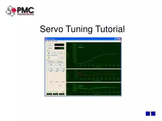
17. Current Position Readout Axis Selector button Motor Enable button & indicator Trajectory Generator Enable & indicator button Move motor buttons Clear plot displays Zero Current Position PID slide control scaling buttons Proportional gain, Integral gain, and Derivative gain slide controls PID filter settings Servo Tuning Program Controls and Indicators Position versus Time plot window Following error versus Time plot window DAC command output versus Time plot window

18. Open plot data point file Reset all settings to default parameters Save plots as a data file Select one of multiple PMC motion controllers Load servo settings from MCAPI.ini file Print step response plots and servo parameters Servo Tuning Program File Menu Options

19. Set and edit servo settings (PID, Vel/Accel/Decel, Trapezoidal/S-curve, Limits, Phasing, etc.) Set User Units Scale PID slider controls Define Step response parameters (Step distance, Plot window time, Position capture delay) Define plot window appearance Servo Tuning Program Setup Menu Options

20. From the Setup Menu open the Servo Setup Dialog box Over Travel Limits should be enabled Not applicable at this time PID Loop Rate should be set to High Typical Derivative Sampling Period is 0.00075 seconds. For high inertia/low friction servo systems the Derivative Sampling period should be between 0.00125 to 0.002 seconds. Not applicable at this time Getting Started Step #1 - Verifying Servo Setup Parameters

21. From the Setup Menu open the Test Setup Dialog box Define a position capture delay time. A non zero value delays the capturing of position data by n milliseconds. This feature is typically used to zoom in and observe in detail how well the axis settles at the target. For now leave this value at 0. Set the Step Response distance. Typical distance is 100 encoder counts. Set the Plot window time base (position record time). Typical time is 500 milliseconds. Select Plot Torque to enable the DAC output plot window Step #2 – Set the Step Response distance and Plot window setup

22. D upper limit equals 1.56% I upper limit equals 0.2% P upper limit equals 3.13% P slide control upper limit I slide control upper limit D slide control upper limit Step #3 – Zoom in on Slide Controls to increase resolution The Servo Tuning program defaults to setting the slide controls to 100% of the maximum gain setting. Leaving the slide control upper limits at 100% will generally result in insufficient slide control resolution. Press the Zoom In (+) button to change the P, I, and D slide control scaling. Select the P slide control zoom button until the upper limit is 3.13%. Set the I slide control upper limit to 0.2%. Set the D slide control upper limit to 1.56%. Please note that these are just recommended initial settings. The final slide control scaling will vary from axis to axis. Slide control scaling is a usability issue, it has no bearing on the performance of the servo system.

23. Step #4 – Set initial PID values Open the Servo Setup Dialog Box and set these initial PID parameters: Proportional gain = 0.05 Derivative gain = 0.0 Derivative Sampling Period = 0.00075 (If high friction system decrease the sampling period to 0.00025. If High inertial system increase the sampling period to 0.0015.) Integral gain = 0.0 Integration Limit = 50 Following Error = 1024

24. Select the On button to turn on the axis (start the PID loop) If no error conditions are present the green light will turn on The Trajectory Generator must be off. The values for proportional and derivative gains must be determined when moving with just P and D control. In other words no velocity profile (max. velocity or ramping). When the Trajectory Generator is on all moves will use either Trapezoidal or S-curve velocity profiles. Step #5 – Enable the axis

25. Captured actual positions of the axis Select the Step button to move. Captured DAC output Step #6 – Executing the first move Selecting either of the Step buttons will cause the controller to attempt to move the motor. The captured actual positions of the axis are displayed in the upper plot window. The DAC (torque/velocity command) output of the controller is displayed in the lower plot window. Since the Trajectory Generator is off there will be no following error plot (middle plot window).

26. This servo system is much more responsive. With the same proportional gain setting (0.05) the axis crosses the target more than three times. The proportional gain is too high. Step #7 – Setting the Proportional Gain The goal is to find a proportional gain setting that causes the axis to get to, and then cross the target 3 times (no more and no less). Any combination of Step Plus and or Step Minus moves is OK. For this servo system a proportional gain setting of 0.05 is too low. The axis never reaches the target position (100).

27. Motor LED changes from green to red If the Motor LED turns red and the motor moves in the wrong direction (negative command output results in more negative encoder counts) the axis is reversed phased. The phasing can be changed in software by selecting the Reverse Phase box in the Servo Tuner, Axis Setup dialog box, or by issuing the appropriate MCCL command (PH), or C/C++ function (MCSetOutputPhase()) from your own application application program. For a hardware solution, you can do the same thing by swapping the A and B connections from the encoder to the motion controller.

28. Axis crossed the target three times. Proportional gain value (0.026) is acceptable. Axis crossed the target only twice. Zero the position display, increase proportional gain, and move again Axis crossed the target more than 3 times. Zero the position display, reduce the proportional gain, and move again. Here is a demonstration of the steps typically required to determine the correct proportional gain setting. Axis did not reach the target. Zero the position display, increase the proportional gain, and move again

29. Set the Derivative Sampling Period Step #8 – Setting the Derivative Gain Open the Servo Setup Dialog and verify the setting for the Derivative Sampling Period. The default value (0.000250) can be used for systems with a great deal of friction, but for typical servo systems it is recommended that the sampling period be set to 0.00075 seconds. With this setting the comparison of the change in following error occurs once every 6 PID loops (an interval of .75 milliseconds).

30. Overshoot limit (125) Overshoot = 65% Overshoot = 50% Overshoot = 35% Overshoot = 25%, current derivative gain setting (0.2675) is acceptable Once an appropriate proportional gain value has been selected the axis is observed overshooting the target by about 65%. Use derivative gain to limit this overshoot to approximately 25%. The greater the overshoot, the more responsive the servo but the more likely the axis is to become unstable (oscillate). If the overshoot is reduced too much (less than 10%) the system will be over dampened and the axis will tend to stop short of the target. Here is a demonstration of how the proper derivative gain value is determined Overshoot is greater than 25%, zero the position display, increase derivative gain, and move the axis. Overshoot is greater than 25%, zero the position display, zoom out the derivative slide control, increase derivative gain, and move the axis. Overshoot is greater than 25%, zero the position display, increase derivative gain, and move the axis.

31. Symptoms of an over dampened servo system In the days of slow servo loops (1, 2, and 5 mSec) an over dampened servo was easy to spot. It typically moved slowly towards the target and would stop 5% to 15% short.

32. The processing power of today’s servo controllers provide a significant boost in servo loop rates, which can complicate the identification of an over dampened servo. The step response on the left side is the traditional over dampened servo system. The step response on the right exhibits significant oscillation in the command output and a noise similar to grinding is heard. A quick glance could result in an incorrect assumption, that the proportional gain has been set too high. In fact the gain settings for both step responses are exactly the same (P = 0.025, D=1.13). The only difference is that prior to executing the second step response the Derivative Sampling Period was reduced from 1 millisecond to 0.5 milliseconds. The oscillation was caused by the combination of excessive derivative gain and short derivative sampling period. This combination causes a high performance servo controller to overreact, resulting in a system that appears to have no dampening at all.

33. Set the desired Acceleration and Deceleration rates Set the desired Maximum Velocity Step #9 – Setting the Integral Gain This is when we start to get to the good stuff. As discussed earlier, Integral gain is used to get the axis to the target. Which means that we can now turn on the trajectory generator and start executing actual moves. But first open up the Servo Setup Dialog and define Maximum Velocity, Acceleration, and Deceleration values for the specific application. For this example application the desired maximum velocity is 100,000 encoder counts per second. The acceleration and deceleration rates are 150,000 encoder counts per second per second.

34. Set the desired move distance. This value can be in encoder counts (default units) or user units. Set the plot window time period Now open the Test Setup Dialog and enter the desired move distance and plot window display period. For this example the move distance is 5000 encoder counts and the time period is 500 milliseconds.

35. Zero the position of the servo, turn on the Trajectory Generator and see how the servo performs. Slowly increase the integral gain until the axis is within 1 encoder count of the target (5000) The axis stopped short of the target. Increase the integral gain until the axis is within 1 count of the target. The axis reached and settled within 1 count of the target. The servo is now tuned. Axis is now within 1 encoder count of the target. Execute a move. Axis is now within 1 encoder count of the target. Execute a move. If increasing the integral gain fails to get the axis to the target, open the Servo Setup Dialog and increase the Integration Limit.

36. Step #9 – Saving the tuning parameters When the controller is reset or the computer power is cycled, all servo setup parameters are reset to default values. After tuning the axis you need to save the servo setup parameters to a file so that they can be reloaded at anytime. To save all of the values in the Servo Setup Dialog, open the File menu and select Save All Axis Settings. This will save the setup parameters to the MCAPI.INI file (in the Windows folder). These parameters can now be used by any application program that uses PMC’s Motion Control API. When using any PMC application program or demo the setup parameters will be loaded automatically if the File menu option Auto Initialize is selected. To load the MCAPI.INI file setup parameters from a user’s application program call the MCAPI function MCDLG_RestoreAxis( ). For further details please refer to the MCAPI help file Mcdlg.hlp.

37. Axis has settled (following error = 0). Settling time reduced by 145 msec’s to 65 msec’s. Axis has settled (following error = 0). Settling time = 210 msec’s. Trajectory complete: after 440 msec’s the calculated optimal position = the move target (5000). Trajectory complete: after 440 msec’s the calculated optimal position = the move target (5000). Analyzing the performance of the servo Once the servo is tuned, the capture delay feature can be used to zoom in on a specific segment of a move. In this example the settling time is of significant importance. By delaying the capturing of positions by 400 milliseconds, and decreasing the plot window time period from 0.5 seconds to 0.3 seconds, the user can analyze how well the axis settles at the target. The settling time can be reduced by: 1) Reducing the Integral gain and 2) Increasing the Proportional gain

38. Visit us on the web at www.pmccorp.com This is the end of the: Servo Tuning Tutorial presentation