Download
1 / 32
320 likes | 407 Views
Comparison of L and P band radar time series for the monitoring of Sahelian area. P.-L. Frison, G. Mercier, E. Mougin, P. Hiernaux. Context : Better understanding Sahelian surface processes and their interaction with monsoon variability

E N D
Comparison of L and P band radar time series for the monitoring of Sahelian area P.-L. Frison, G. Mercier, E. Mougin, P. Hiernaux
Context: BetterunderstandingSahelian surface processes and their interaction withmonsoonvariability Improveourunderstanding and documentation of long term trend in vegetation in response to climate change radar data: 2 keyparameters: soilmoisture and vegetation Goal: Comparison of L band PALSAR and C band ASAR data for Sahelian surface monitoring. Relation between radar vs surface parameter temporal evolution
Outline: • Study site • PALSAR and ASAR data • change detectionmethod • Results and discussion
The Sahel Dry season (Nov. – Apr.) bare soil Semi-arid area shrub (0-20 %) trees (1-5 %) + Rainy season (May – Oct.) herbaceous layer (0-50 %) (annual grasses)
Region of study: the Gourma - Mali Seno
DATASET PALSAR acquisitions: L band (Jan. 2007 - Apr. 2009) ASAR acquisitions: C band (Jul. - Dec. 2005)
Gourma Region (MALI) ASAR –Wide Swath - HH 20th Dec 2005
GOURMA Region (MALI) PALSAR–WIDE BEAM- HH 1st Jan 2008
ASAR C-band Gourma Region (MALI) PALSAR L-band C-band (ASAR): Shallow sand and silt soils L -band (PALSAR): Better discrimination of geological features Remnant of alluvial systems and lacustrine depressions
ASAR C-band Gourma Region (MALI) PALSAR L-band C-band (ASAR): Shallow sand and silt soils L -band (PALSAR): Better discrimination of geological features Remnant of alluvial systems and lacustrine depressions
PALSAR Fine Beam – HH polarization Temporal color composite image Water ponds Hombori mounts Low-land (accacia forest) 17 Jan. 2007 20 Oct. 2007 22 Jan.2009 GOURMA - MALI
Change detection method Constraints: Large dynamic range (high differences over bright patterns) Even after multi-looking, presence of noise (speckle) absolute or relative differences, ratios, rms,….. not significant Time seriescolor composite image Relative differences
Change detection method Constraints: Large dynamic range (high differences over bright patterns) Even after multi-looking, presence of noise (speckle) absolute or relative differences, ratio, rms,….. not significant Case of 3 channels Temporally stable regions gray Change detection colored areas
Change detection method Constraints: Large dynamic range (high differences over bright patterns) Even after multi-looking, presence of noise (speckle) absolute or relative differences, ratio, rms,….. not significant Case of 3 channels Temporally stable areas gray areas (no saturation) Change detection colored areas (saturation) Value B Hue G 0 Saturation R RGB space HSV space
RGB Space 17 Jan. 2007 20 Oct. 2007 22 Jan.2009
Value HSV Space Saturation Hue Areas that have changed
Change detection for a 3-date color composite image Saturation image Color composite image 17 Jan. 2007 20 Oct. 2007 22 Jan.2009 PALSAR Fine Beam HH polarization
Change detection method Case of N channels (N>3): P iterations: 1) random draw of 3 among the N available channels 2) Compute the saturation channel from HSV space Average of the P saturation channels Example: 12 Finebeam acquisitions at HH pol. N=12 12! / (9! * 3!) = 220 possible random draws P =50 (arbitrary)
Change detection for a 3-date color composite image Saturation image Color composite image 17 Jan. 2007 20 Oct. 2007 22 Jan.2009 PALSAR Fine Beam HH polarization
Change detection for 12 FineBeam acquisitions (HH polarization) Saturation image Color composite image 17 Jan. 2007 20 Oct. 2007 22 Jan.2009 Jan. 2007 – Apr. 2009 PALSAR Fine Beam HH polarization
Temporal changes detected over 12 Fine Beam acquisitions Water ponds Fields (millet) dep. Orientation! PALSAR data HH polarisation Jan. 2007 – Mar. 2009 Significant penetration depth over sandy soils
Temporal changes detected over 12 Fine Beam acquisitions Water ponds permanent Fields (millet) dep. Orientation! PALSAR data HH polarisation Jan. 2007 – Mar. 2009 Changes in dry season Changes in rainy season
INFLUENCE OF POLARISATION Sandy soils Shallow soils HH HV ALOS/PALSAR – FBD 6th June 2008
Change detection between HH and HV Shallow soils + Water ponds PALSAR DUAL POLARIZATION
ALOS/PALSAR – WB1: HH Polarization 3-date color composite image Water ponds discrimination 2008 dry season: 1 Jan 16 Feb 2 Apr
ALOS/PALSAR – WB1: HH Polarization Change detection (dry season) • Water pondsdiscrimination • Main water resource • Hydrological indicator • surface runoff • areas increase since begining of drought period (50’s)
ASAR –Wide Swath – HH polarisation • 41 acquisitions • 22 acquisitions in ascending pass • 5 acquisitions same incidence angle (35°) – Jul. –Dec. 2005
ASAR –Wide Swath - HH polarisation change detection (5 dates) 2nd Sept. 2005 low penetration over sandy soil upper surface changes sandy soils
ASAR –Wide Swath - HH polarisation change detection (5 dates) 2nd Sept. 2005 low penetration over sandy soil upper surface changes sandy soils, water ponds
Comparison P band / L band temporal change detection PALSAR (L-band) change detection (5 dates) High penetration dpeth over sandy soils water ponds millet fields low penetration over sandy soil upper surface changes sandy soils, water ponds
Conclusion • RGB HSV simple but performant for change detection ! histogram must be the same across the hole image! • Temporal change detection: penetration depth illustration L band (high penetration over sandy soils) Water ponds Millet fields • C band (low penetration over sandy soils) • mix of upper surface changes • sandy soils (soil moisture + vegetation) • water ponds • more difficult te discriminate special features • L band: some variation over sandy soils (soil moisture?) • Cross over with SMOS mission