Walter N. Meier, Melinda Marquis, Marilyn Kaminski,

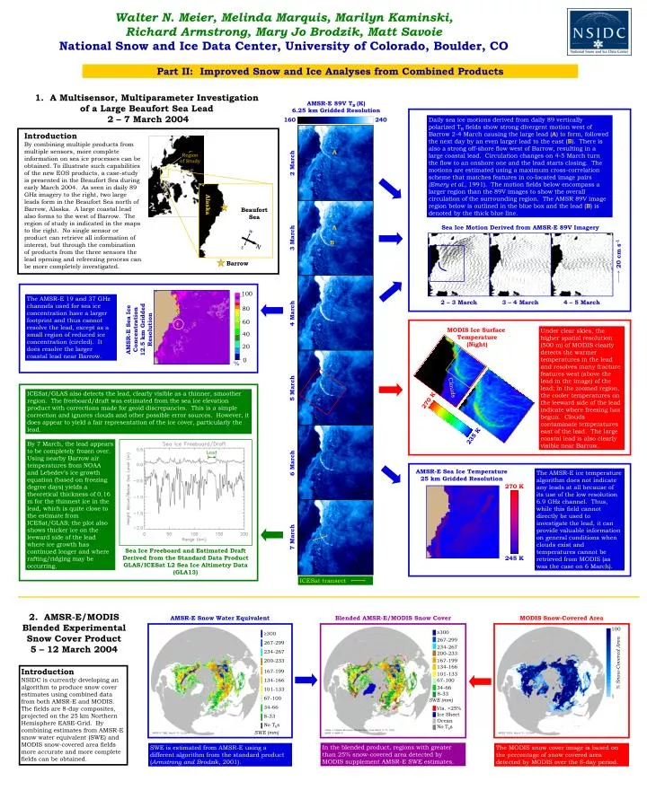
1. Alaska Beaufort Sea W N 270 K E Barrow 235 K 100 80 60 40 20 0 % Lead Walter N. Meier, Melinda Marquis, Marilyn Kaminski, Richard Armstrong, Mary Jo Brodzik, Matt Savoie National Snow and Ice Data Center, University of Colorado, Boulder, CO Part II: Improved Snow and Ice Analyses from Combined Products 1. A Multisensor, Multiparameter Investigation of a Large Beaufort Sea Lead 2 – 7 March 2004 AMSR-E 89V TB (K) 6.25 km Gridded Resolution 160 240 Daily sea ice motions derived from daily 89 vertically polarized TB fields show strong divergent motion west of Barrow 2-4 March causing the large lead (A) to form, followed the next day by an even larger lead to the east (B). There is also a strong off-shore flow west of Barrow, resulting in a large coastal lead. Circulation changes on 4-5 March turn the flow to an onshore one and the lead starts closing. The motions are estimated using a maximum cross-correlation scheme that matches features in co-located image pairs (Emery et al., 1991). The motion fields below encompass a larger region than the 89V images to show the overall circulation of the surrounding region. The AMSR 89V image region below is outlined in the blue box and the lead (B) is denoted by the thick blue line. Introduction By combining multiple products from multiple sensors, more complete information on sea ice processes can be obtained. To illustrate such capabilities of the new EOS products, a case-study is presented in the Beaufort Sea during early March 2004. As seen in daily 89 GHz imagery to the right, two large leads form in the Beaufort Sea north of Barrow, Alaska. A large coastal lead also forms to the west of Barrow. The region of study is indicated in the maps to the right. No single sensor or product can retrieve all information of interest, but through the combination of products from the three sensors the lead opening and refreezing process can be more completely investigated. A Region of Study 2 March A Sea Ice Motion Derived from AMSR-E 89V Imagery 3 March B 20 cm s-1 The AMSR-E 19 and 37 GHz channels used for sea ice concentration have a larger footprint and thus cannot resolve the lead, except as a small region of reduced ice concentration (circled). It does resolve the larger coastal lead near Barrow. 2 – 3 March 3 – 4 March 4 – 5 March 4 March AMSR-E Sea Ice Concentration 12.5 km Gridded Resolution MODIS Ice Surface Temperature (Night) Under clear skies, the higher spatial resolution (500 m) of MODIS clearly detects the warmer temperatures in the lead and resolves many fracture features west (above the lead in the image) of the lead; in the zoomed region, the cooler temperatures on the leeward side of the lead indicate where freezing has begun. Clouds contaminate temperatures east of the lead. The large coastal lead is also clearly visible near Barrow. Clouds 5 March ICESat/GLAS also detects the lead, clearly visible as a thinner, smoother region. The freeboard/draft was estimated from the sea ice elevation product with corrections made for geoid discrepancies. This is a simple correction and ignores clouds and other possible error sources. However, it does appear to yield a fair representation of the ice cover, particularly the lead. By 7 March, the lead appears to be completely frozen over. Using nearby Barrow air temperatures from NOAA and Lebedev’s ice growth equation (based on freezing degree days) yields a theoretical thickness of 0.16 m for the thinnest ice in the lead, which is quite close to the estimate from ICESat/GLAS; the plot also shows thicker ice on the leeward side of the lead where ice growth has continued longer and where rafting/ridging may be occurring. 6 March AMSR-E Sea Ice Temperature 25 km Gridded Resolution The AMSR-E ice temperature algorithm does not indicate any leads at all because of its use of the low resolution 6.9 GHz channel. Thus, while this field cannot directly be used to investigate the lead, it can provide valuable information on general conditions when clouds exist and temperatures cannot be retrieved from MODIS (as was the case on 6 March). 270 K 7 March Sea Ice Freeboard and Estimated Draft Derived from the Standard Data Product GLAS/ICESat L2 Sea Ice Altimetry Data (GLA13) 245 K ICESat transect 2. AMSR-E/MODIS Blended Experimental Snow Cover Product 5 – 12 March 2004 AMSR-E Snow Water Equivalent Blended AMSR-E/MODIS Snow Cover MODIS Snow-Covered Area 100 ≥300 ≥300 267-299 267-299 234-267 234-267 200-233 167-199 200-233 % Snow-Covered Area 134-166 Introduction NSIDC is currently developing an algorithm to produce snow cover estimates using combined data from both AMSR-E and MODIS. The fields are 8-day composites, projected on the 25 km Northern Hemisphere EASE-Grid. By combining estimates from AMSR-E snow water equivalent (SWE) and MODIS snow-covered area fields more accurate and more complete fields can be obtained. 167-199 101-133 134-166 67-100 34-66 101-133 8-33 1 67-100 SWE (mm) 34-66 Vis. >25% Ice Sheet 8-33 Ocean No Tbs No Tbs SWE (mm) In the blended product, regions with greater than 25% snow-covered area detected by MODIS supplement AMSR-E SWE estimates. SWE is estimated from AMSR-E using a different algorithm from the standard product (Armstrong and Brodzik, 2001). The MODIS snow cover image is based on the percentage of snow covered area detected by MODIS over the 8-day period.