Download
1 / 44
440 likes | 521 Views
9. Linear Regression and Correlation. Data: y: a quantitative response variable x: a quantitative explanatory variable (Chap. 8: Recall that both variables were categorical ) For example (Wagner et al., Amer. J. Community Health , vol. 16, p. 189)

E N D
9. Linear Regression and Correlation Data: y: a quantitative response variable x: a quantitative explanatory variable (Chap. 8: Recall that both variables were categorical) For example (Wagner et al., Amer. J. Community Health, vol. 16, p. 189) y = mental health, measured with Hopkins Symptom List (presence or absence of 57 psychological symptoms) x = stress level (a measure of negative events weighted by the reported frequency and subject’s subjective estimate of impact of each event) We consider: • Is there an association? (test of independence) • How strong is the association? (uses correlation) • How can we describe the nature of the relationship, e.g., by using x to predict y? (regression equation, residuals)
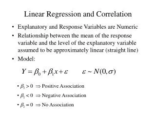
Linear Relationships Linear Function (Straight-Line Relation): • y = a + b x • expresses y as linear function of x with slope b and y-intercept a. For each 1-unit increase in x, y increases b units b > 0 Line slopes upward b = 0 Horizontal line b < 0 Line slopes downward
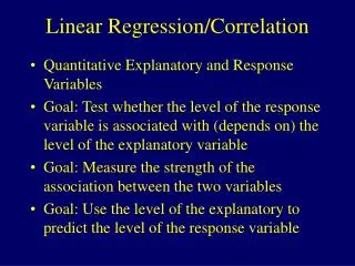
Example: Economic Level and CO2 Emissions OECD (Organization for Economic Development, www.oecd.org): Advanced industrialized nations “committed to democracy and the market economy.” oecd-data file (from 2004) on p. 62 of text and at text website www.stat.ufl.edu/~aa/social/ • Let y = carbon dioxide emissions (per capita, in metric tons) Ranges from 5.6 in Portugal to 22.0 in Luxembourg mean = 10.4, standard dev. = 4.6 • x = GDP (thousands of dollars, per capita) Ranges from 19.6 in Portugal to 70.0 in Luxembourg mean = 32.1, standard dev. = 9.6
The relationship between x and y can be approximated by y = 0.42 + 0.31x. • At x = 0, predicted CO2 level y = • At x = 39.7 (value for U.S.), predicted CO2 level y = (actual = 19.8 for U.S.) • For each increase of 1 thousand dollars in per capita GDP, CO2 use predicted to increase by metric tons per capita • But, this linear equation is just an approximation, and the correlation between x and y for the OECD nations was 0.64, not 1.0. Scatterplot on next page.
Effect of variable coding? Slope and intercept depend on units of measurement. • If x = GDP measured in dollars (instead of thousands of dollars), then y = because a change of $1 has only 1/1000 the impact of a change of $1000 (so, the slope is multiplied by 0.001). • If y = CO2 output in kilograms instead of metric tons (1 metric ton = 1000 kilograms), with x in dollars, then y = Suppose x changes from U.S. dollars to British pounds and 1 pound = 2 dollars. What happens?
Probabilistic Models • In practice, the relationship between y and x is not “perfect” because y is not completely determined by x. Other sources of variation exist. • We let a + bx represent the mean of y-values, as a function of x. • We replace equation y = a + bx by E(y) = a + bx (for population) (Recall E(y) is the “expected value of y”, which is the mean of its probability distribution.) e.g., if y = income, x = no. years of education, we regard E(y) = a + b(12) as the mean income for everyone in population having 12 years education.
A regression function is a mathematical function that describes how the mean of the response variable y changes according to the value of an explanatory variable x. • A linear regression function is part of a model (a simple representation of reality) for summarizing a relationship. • In practice, we use data to check whether a particular model is plausible (e.g., by looking at a scatterplot) and to estimate model parameters.
Estimating the linear equation • A scatterplot is a plot of the n values of (x, y) for the n subjects in the sample • Looking at the scatterplot is first step of analysis, to check whether linear model seems plausible Example: Are externalizing behaviors in adolescents (e.g., acting out in negative ways, such as causing fights) associated with feelings of anxiety? (Nolan et al., J. Personality and Social Psych., 2003)
Data (some) Subject Externalizing (x) Anxiety (y) 1 9 37 2 7 23 3 7 26 4 3 21 5 11 42 6 6 33 7 2 26 8 6 35 9 6 23 10 9 28 As exercise, conduct analyses with x, y reversed
Variables • Anxiety (y) Externalizing (x) • mean 29.4 6.6 • std. dev.7.0 2.7
How to choose the line that “best fits” the data? • Criterion: Choose line that minimizes sum of squared vertical distances from observed data points to line. This is called the least squares prediction equation. Solution (using calculus): Denote estimate of by a, estimate of by b, estimate of E(y) and the prediction for y by . Then, with
Example: What causes b > 0 or b < 0? Subject Externalizing (x) Anxiety (y) 1 9 37 2 7 23 Numerator of b is The contribution of subjects 1 and 2 to b is
Motivation for formulas: • If observation has both x and y values above means, or both values below means, then (x - )(y - ) is positive. Slope estimate b > 0 when most observations like this. • means that • i.e., predicted value of y at mean of x is mean of y. The prediction equation passes through the point with coordinates ( , ).
Results for anxiety/externalizing data set Least squares estimates are a = 18.407 and b = 1.666. That is,
Interpretations • 1-unit increase in x corresponds to predicted increase of in anxiety score. • y-intercept of is predicted anxiety score for subject having x = . • The value b = corresponds to a positive sample association between the variables. • … but, sample size is small, with lots of variability, and it is not clear there would be a positive association for a corresponding population.
Residuals (prediction errors) • For an observation, difference between observed value of y and predicted value of y, is called a residual (vertical distance on scatterplot) Example: Subject 1 has x = 9, y = 37. Predicted anxiety value is Residual = = Residual positive when Residual negative when The sum (and mean) of the residuals = 0.
Prediction equation has “least squares” property • Residual sum of squares (i.e., sum of squared errors): • The “least squares” estimates a and b provide the prediction equation with minimum value of SSE • For software tells us SSE = . Any other equation, such as has a larger value for SSE.
The Linear Regression Model • Recall the linear regression model is E(y) = + x (probabilistic rather than deterministic). • The model has another parameter σ that describes the variability of the conditional distributions. • The estimate of the conditional standard deviation of y is
Example: We have SSE = 254.2 based on n = 10. At any fixed level of x, the estimated standard deviation of anxiety values is (Called “Std. Error of the Estimate” in SPSS printout)
df = n – 2 is degrees of freedom for the estimate s of σ. (n – 2 because … ) • The ratio SSE/(n-2)is called the mean square error and often denoted by MSE. • The total sum of squares about the sample mean of y decomposes into the sum of the residual (error) sum of squares and the regression sum of squares TSS = SSE + Regression SS We’ll see that regression is more effective in predicting y using x when SSE is relatively small, regression SS is relatively large.
Software shows sums of squares in an “ANOVA” (analysis of variance) table
Example: (text, p. 267, study in undergraduate research journal by student at Indiana Univ. of South Bend) • Sample of 50 college students in an introductory psychology course reported y = high school GPA and x = weekly number of hours watching TV • The study reported • Software reports: ---------------------------------------------------------------------------- Sum of Squares df Mean Square Regression 3.63 1 3.63 Residual 11.66 48 .24 Total 15.29 49 -----------------------------------------------------------------------------
The estimate of the conditional std dev is i.e., predict GPA’s vary around 3.44 – 0.03x with a standard deviation of e.g., at x = 10 hours of TV watching, conditional dist of GPA is estimated to have mean of and a standard deviation of . Note: Conditional std. dev. s differs from marginal std. dev. of y, which ignores x in describing variability of y (Normally cond. std. dev. s < marginal std. dev. sy )
Example: y = GPA, x = TV watching We found s = 0.49 for estimated conditional standard deviation of GPA Estimated marginal standard deviation of GPA is How can they be dramatically different? (picture)
Measuring association: The correlation • Slope of regression equation describes the direction of association between x and y, but… • The magnitude of the slope depends on the units of the variables • The correlation is a standardized slope that does not depend on units • Correlation r relates to slope b of prediction equation by r = b(sx/sy) where sxand sy are sample standard deviations of x and y.
Properties of the correlation • r is standardized slope in sense that r reflects what b equals if sx = sy • -1 ≤ r ≤ +1, with r having same sign as b • r = 1 or -1 when all sample points fall exactly on prediction line, and r describes strength of linear association • r = 0when b = 0 • The larger the absolute value, the stronger the assoc.
Examples • For y = anxiety and x = externalizing behavior, = 18.41 + 1.67x, and sx = 2.7, sy = 7.0. The correlation equals r = b(sx/sy) = • For y = high school GPA and x = TV watching, we’ll see that r = - 0.49 (moderate negative association) • Beware: Prediction equation and r can be sensitive to outliers
Correlation implies that predictions regress toward the mean • When x goes up 1, predicted y changes by b • When x goes up sx, thepredicted y changes by sxb = rsy A 1 standard deviation increase in x corresponds to predicted change of r standard deviations in y. y is predicted to be “closer” to its mean than x is to its mean; i.e., there is regression toward the mean (Francis Galton 1885) Example: x = parent height, y = child height
r2 = proportional reduction in error • When we use x in the prediction equation to predict y, a summary measure of prediction error is sum of squared errors • When we predict y without using x, best predictor is sample mean of y, and summary measure of prediction error is total sum of squares Predictions using x get “better” as SSE decreases relative to TSS
The proportional reduction in error in using x to predict y (via the prediction equation) instead of using sample mean of y to predict y is • i.e., the proportional reduction in error is the square of the correlation! • This measure is sometimes called the coefficient of determination, but more commonly just “r-squared”
Example: high school GPA and TV watching Sum of Squares df Mean Square Regression 3.63 1 3.63 Residual 11.66 48 .24 Total 15.29 49 So, r2 = There is a % reduction in error when we use x = TV watching to predict y = high school GPA. “ % of the variation in high school GPA is explained by TV watching.” The correlation r is
Properties of r2 • Since -1 ≤ r ≤ +1, 0 ≤ r2 ≤ 1 • Minimum possible SSE = 0, in which case r2 = 1and all sample points fall exactly on prediction line • If b = 0, then so and so TSS = SSE and r2 = 0. • r2 does not depend on units, or distinction between x, y
Inference about slope (b) and correlation () Assumptions: • The study used randomization in gathering data • The linear regression equation E(y) = + x holds • The standard deviation σ of the conditional distribution is the same at each x-value. • The conditional distribution of y is normal at each value of x (least important, especially for two-sided inference with relatively large n)
Test of independence of x and y • Parameter: Population slope in regression model(b) • Estimator: Least squares estimate b • Estimated standard error: decreases (as usual) as n increases • H0: independence is H0: = 0 • Ha can be two-sided Ha: 0 or one-sided, Ha: > 0 or Ha: < 0 • Test statistic t = (b – 0)/se, with df = n – 2
Example: Anxiety/externalizing behavior revisited From SPSS output below, t = , df = n – 2 = , two-sided P-value = . Considerable evidence against H0: = 0. It appears there is positive association in population between externalizing behaviors and feelings of anxiety. For Ha: > 0, P-value = right-tail probability above t = 2.41, which is
Confidence interval for slope • A CI for has form b ± t(se) where t-score has df = n-2 andis from t-table with half the error probability in each tail. Example: b = 1.666, se = 0.692 With df = 8, for 95% CI, t-score = 95% CI for is 1.666 ± We conclude that association in population is positive, with slope in this range (wide CI because n so small) (Recall y = anxiety has mean = 29, std. dev. = 7 x = externalizing behavior has mean = 6.6, std. dev. = 2.7)
What is effect of 3-unit increase in x = externalizing behavior?(nearly a standard deviation increase in x) Estimate is now 3b, which has 3(se), and we have • Conclusion of two-sided test about H0: = 0 is consistent with conclusion of corresponding CI, with error prob. that is the significance level of test. Example: Two-sided P-value = 0.04, so reject H0: = 0 at 0.05 level and conclude there is an association. Likewise, 95% CI for does not contain 0 as a plausible value for .
What if reverse roles of variables?(Now, y = externalizing behavior, x = anxietyPrediction equation changes Correlation stays same Result of t test is same
Some comments • Equivalent test of independence uses H0: = 0, where is popul. correlation that sample correlation r estimates Test statistic Example: r = 0.648, n = 10, so t = 0.648/0.269 = 2.41, df = 8. P-value = 0.043 for Ha : 0. • CI for more complex because of skewed sampling distribution
Linear regression is a model: We don’t truly expect exactly a linear relation with constant variability, but it is often a good and simple approximation in practice. • Extrapolation beyond observed range of x-values dangerous. For y = high school GPA and x = weekly hours watching TV, . If observe x between 0 and 30, say, does not make sense to plug in x=100and get predicted GPA = 0.44. • Observations are very influential if they take extreme values (small or large) of x and fall far from the linear trend the rest of the data follow. These can unduly affect least squares results.
Example of effect of outlier • For data on y = anxiety and x = externalizing behavior, subject 5 had x = 11, y = 42. Suppose data for that subject had been incorrectly entered in data file as x = 110 and y = 420. • Instead of = 18.41 + 1.67x, weget = • Instead of r = 0.64, get r = • Suppose x enteredOKbut y entered as 420. Then = , and r = .
Correlation biased downward if only narrow range of x-values sampled. (see picture) Example (p. 286): How strong is association between x = SAT exam score and y = college GPA at end of second year of college? We’ll find a very weak correlation if we sample only Harvard students, because of the very narrow range of x-values. • An alternative way of expressing the model E(y) = + x is y = + x + , where is a population residual (error term) that varies around 0 (see p. 287 of text)
Software reports SS values, test results in an ANOVA (analysis of variance) tableThe F statistic in the ANOVA table is the square of the t statistic for testing H0: = 0, and it has the same P-value as for the two-sided test. This is a more general statistic that we’ll need when a hypothesis contains more than one regression parameter (Chap. 11).