Download
1 / 145
1.74k likes | 2.93k Views
Doppler Radar. The Doppler Effect The Doppler Dilemma Etc – other topics Doppler Analysis and Diagnosis (Important New and Original Material linked to slide 80). The Doppler effect. Classically, the Doppler effect is a frequency shift

E N D
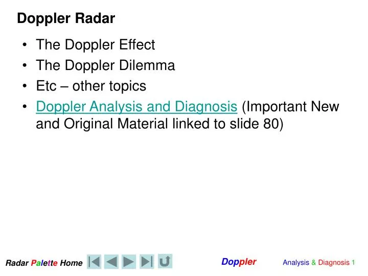
Doppler Radar • The Doppler Effect • The Doppler Dilemma • Etc – other topics • Doppler Analysis and Diagnosis (Important New and Original Material linked to slide 80)
The Doppler effect • Classically, the Doppler effect is a frequency shift • The change in frequency of a signal returned from a target owing to its radial motion relative to an observer • With radar, this is measured as a shift in phase between the transmitted pulse and the backscattered microwave radiation • Average radial velocity of the target is calculated from this phase shift
Velocity Spectrum Stationary GC WX WX Moves -VN 0 +VN
Phase Shift Ambiguity A shift of ¼ wavelength is ambiguous. You don’t know if your are coming or going?
Velocity folding – Phase Shift Ambiguity • Target radial velocities producing phase shifts greater than one-half wavelength (or p radians) results in velocity folding • Maximum unambiguous radial velocity Vmax (Nyquist velocity) = • (PRF X Wavelength)/ 4 • This range is not adequate to describe all horizontal velocities Nyquist velocity=1200 X 5cm/4 = 1500cm/sec=15m/s=30knots Is a Nyquist velocity of 30knots enough?
The velocities with this storm are HUGE !!!! Quick, increase the PRF and give me a sector scan on the storm cell ! Vmax (Nyquist velocity) = (PRF X Wavelength) / 4 By increasing the PRF, velocity foldng starts at a higher radial velocity
Folded Doppler quickly reaches the maximum colour range and cycles to opposite colours = noisy, complicated fields Interpretation is challenging! Helen was right! ? ? After PRF increased Before Helen’s Demand
Doppler Dilemma • Maximum unambiguous range: • Rmax = c / 2PRF • What is this for PRF = 1200 ? • VmaxRmax = cl/8 • Vmax and Rmax are inversely proportional to each other, but we want to maximize both • That’s the Doppler dilemma 125 km
Velocity Unfolding • Use two PRF’s and take the difference in the Doppler velocities ! • The difference turns out to be a unique function of the actual velocity out to much higher velocities!! • So DV and one of the velocity measurements can be used to unambiguously calculate the actual radial velocity, perhaps up to 48 m/s (almost 100 knots).
Now we can see the whole storm, Bill ! That’s great, Jo. Now if only Dorothy and pigs would fly !
Example: Radial Velocity Product with Vr to 48 m/s N-S Warm Front? Katabatic Cold Front? WLY upper level winds SELY low level winds
Doppler wind interpretation • You can determine wind direction vs. height away from radar in two different directions • Go out along zero line • Draw line back to radar • Wind is perpendicular to this line, towards the red echoes
Doppler wind interpretation • For any height you can attempt to determine the wind in 4 locations • Determine the two zero line winds • Look roughly 90° away for the max wind, which should be all directed along a radial • In this way you can see areas of non-uniform flow • confluence, diffluence
Doppler Uniform 30 m/s wind everywhere
Doppler Display - Uniform Wind Shear Vertical Wind Shear of 13 knots per kilometre = Speed Shear only
20 20 Doppler with Directional Shear and Jet Directional Shear and Wind Maximum
Doppler with Wind Shear - Speed and Directional Direction veering with height Speed increasing with height
Doppler Practice Westerly Winds with only Speed shear
Doppler Practice Westerly Winds with Low Level Jet
Doppler Practice Veering Winds with no Speed shear
Doppler Practice Backing Winds with no Speed shear
Doppler Practice Changes in Stability? Low Level Veering under High Level Backing Winds - no Speed shear
Doppler Practice Wind shift line
Doppler Practice Large Scale Convergence
Doppler Practice Radar Site Divergence
Doppler Practice Radar Site Cyclonic Vortex
SWLY NNELY Doppler Practice LLJ QS Horizontal LLJ Marginal winds Backing with Height - Cold Air Advection Maybe a Cold Conveyor Belt ahead of a synoptic system…
Velocity Azimuth Display - VAD • Doppler radial velocity data used to construct a wind profile in the vertical • Direction, speed (m/s) and reflectivity (dBZ) displayed as a function of height (km) • Note: Velocity scale is fixed in range 0-20 m/s ( i.e. most of the unfolded velocities are not used )
Velocity Azimuth Display - VAD • At a given height (h), then the radial velocity is: • For a uniform flow field and assume Vw (Vertical Velocity) approximately = 0 then • Best fit of a sine curve to the observations around the circle.
Velocity Azimuth Display - VAD • Accuracy of VAD decreases with elevation angle and height. The desired horizontal wind component becomes a smaller part of the radial wind component actually measure. • Errors in the radial component has a bigger impact on the accuracy of the horizontal wind
A new Velocity Azimuth Display LOLAA sees winds far from radar 3.5° scan sees winds closer in to radar – behaves most like a “profiler”
Doppler Spectra Width • Spread of the Doppler Power Spectrum • the spread, range of terminal fall speeds of the scatterers (more pronounced for rain than for snow) spectra for rain spectra for snow • turbulence of the air (upper levels in severe convection) • vertical wind shear (e.g., along a gust front) • antenna motion Rain Snow
Doppler Image Characteristics Small Spectral Width Large Spectral Width
Spectral Width and “Doppler Display Texture” Rain Texture Snow Texture
The Doppler Precipitation Spectral Width Doppler Precipitation Texture Example
The Doppler Twist Signature - Example • The white dashed line separates different wind regimes in the vertical. • It also separates regimes of differing Doppler texture. • Above the dashed line the Doppler texture is uniform and characteristic of snow. • Below the dashed line the texture is lumpy like oatmeal and characteristic of rain. • This is also an example of the Virga Hole Signature The dashed line is likely the warm front. The layer immediately below is where the snow is melting into rain.
Second Trip Echo – Extending the Range of the Doppler Scan Random Phase Processing extends the Doppler Range Dual PRF’s extends the Nyquist Velocity
Second Trip Echo The velocity signatures of second trip echoes are very noisy. These still contribute to the reflectivity signal where they should not.
Second Trip Processing Doppler Reflectivity with Processed Second Trip Echoes Conventional CAPPI Doppler Reflectivity with Second Trip Echoes Doppler Reflectivity