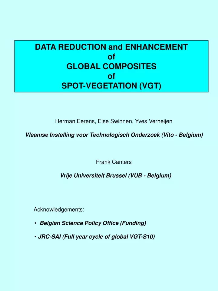
DATA REDUCTION and ENHANCEMENT of GLOBAL COMPOSITES of SPOT-VEGETATION (VGT)

1. DATA REDUCTION and ENHANCEMENT of GLOBAL COMPOSITES of SPOT-VEGETATION (VGT) • Herman Eerens, Else Swinnen, Yves Verheijen • Vlaamse Instelling voor Technologisch Onderzoek (Vito - Belgium) • Frank Canters • Vrije Universiteit Brussel (VUB - Belgium) • Acknowledgements: • Belgian Science Policy Office (Funding) • JRC-SAI (Full year cycle of global VGT-S10)

2. Dec Jan 0.75 0.75 Amazonas Nov Feb 0.50 Oct 0.25 Mar Nile Delta NOAA-AVHRR: 365 x S1 SPOT-VEGETATION: 36 x S10 Sep Apr Sahara Aug May Sahel July June MVC-Composites: - still affected by clouds, bidirectional effects, measurement errors - best visible / removable in longitudinal analysis(time series) - cleaning procedures: MVC-month, BISE, Verhoef,...

3. Monthly Mean NDVI t1 t2 t3 0.8 Max = 0.7 NDVI2 = Min + 0.8(Max – Min) = 0.6 NDVI1 = Min + 0.2(Max – Min) = 0.3 Min = 0.2 0.7 0.6 0.5 0.4 0.3 0.2 0.1 39 12 36 9 24 27 33 3 6 15 18 21 0 30 Decades 0 Extraction of Phenological Variables: - Simple: Annual mean / min / max / amplitude of NDVI - Complex: start / end / length of green season(s) - Often better inputs for classification - Only feasible through longitudinal analysis(time series)

4. Mean Annual NDVI Seasonality Index SI SI = [Range - Mean]/ [Range + Mean] Phenological Variables: Examples from the “Global Land 1km AVHRR Data Set” April 1992 - March 1993, Interrupted Goode Homolosine

5. None (desert/ice) Intermediate Length of Green Season Entire year January June December Start of Green Season No Growing Season Phenological Variables: Examples from the “Global Land 1km AVHRR Data Set” April 1992 - March 1993, Interrupted Goode Homolosine

6. <0.25 <0.25 <0.5 <0.5 >0.5 >0.5 range range <0.1 <0.1 mean mean < 0.17 < 0.17 < 0.35 < 0.35 < 0.45 < 0.45 < 0.55 < 0.55 > 0.55 > 0.55 Phenological Variables: Examples from the “Global Land 1km AVHRR Data Set” April 1992 - March 1993, Interrupted Goode Homolosine Simple Biome Classification Bivariate Level Slice: - Annual Mean NDVI - Annual NDVI Range

7. LONGITUDINAL TIME SERIES ANALYSIS REQUIRED • It adds a new dimension to the results of the transversal analysis (per decade / day) • At a given moment, áll information of a full year (36 x S10, 360 x S1) must be available simultaneously Band BPP CONTENTS VGT-SYNTHESIS ------- ------ ----------------- 1 2 BLUE Reflectance 2 2 RED Reflectance 3 2 NIR Reflectance 4 2 SWIR Reflectance 5 1 NDVI 6 1 Zenith angle of sun 7 1 Zenith angle of sensor 8 1 Azimuth angle of sun 9 1 Azimuth angle of sensor 10 1 Status map: errors in 4 bands, land, cloud, snow/ice 11 2 Time grid: minutes between pixel registration and start of synthesis (LOG-file) Total 16 GLOBAL VGT-SYNTHESIS  600 Mb pixels x 16 byte/pix  10 000 Mb  10 Gb FULL YEAR CYCLE S10: 360 Gb S1: 3.6 Tb • TOO MUCH DATA  CLASSICAL SOLUTIONS: • Temporal selection: select limited number of composites • Spectral selection: only NDVI, … • Spatial selection: - Extract/analyse specific study areas • - Work on degraded images

8. DEDICATED SCHEME FOR DATA REDUCTION 1. Radiometric Compression: 16  6 bytes (37.5%) - Eliminate BLUE and NIR - Rescale reflectances from 16 to 8 bit (0-250) RED/SWIR: R = 0%…62.5% in steps of 0.25% NIR: R = 0%…83.3% in steps of 0.33% - Values 251-255: special flags (saturation, error, ...) - Status_out : Cloud + Snow/ice + Day_in_decade - Combine 2 zenith angles in 1 byte (steps of 5°) - Combine 2 azimuths in 1 byte (relative azimuth:0-180°)  Output = 6 Byte-layers 2. Eliminate all the Water Pixels (25%) - 134,134,736 land pixels left  Spatial context lost! - Results stored in Pseudo-Images (PI)  IDL/ENVI-images (Ncol=5000, Nrec=26827) - All spectral (per-pixel) operations still feasible (via IDL/ENVI): time series analysis, classification (!), ... 3. Improved Land/Sea-Mask - VGT-mask: 5-10 sea pixels along coast (too much) - Boreal regions in winter: confused with sea (status map) 4. Conversion to Equal-Area Projection (IGH): - In: Plane carré of VGT (worst projection) at (1/112°)² - Out: Interrupted Goode Homolosine (IGH) at 1x1km²  REDUCTION: ± 10% without LOSS of DATA !  FULL YEAR CYCLE: S10: 36 Gb S1: 360Gb

9. NORMAL IMAGES - Normal format - Land and water PSEUDO-IMAGES - Only land - All in IGH-Projection - Sorted by Region-ID IGH-Y LAT 111122223334444455555566 Country-ID Raster 1 3 PI_ID PI_X PI_Y PI_LON PI_LAT 5 STEP 1a Extract 1 3 5 2 4 6 STEP 1b Inverse IGH-projection 2 4 6 IGH-X LON 0=sea Scan per Pixel SPOT4-VGT Decadal Synthesis - 11 HDF image layers - 16 bytes/pixel - LOG-File (geo-referencing) Pixel Lon/Lat Convert STEP 2 Transversal Reduction Col/Rec in HDF Read HDF's 1 3 11 Input-Values 5 Filter 2 4 6 Output-Values 6 Output PI_RED PI_NIR PI_SWIR PI_THETA PI_AZIM PI_MASK Output Pseudo-Images - 6 per decadal synthesis - 6 bytes/pixel - Repeat for 36 syntheses/year  36 x 6 = 216 pseudo-images STEP 3 Longitudinal Analysis • - Normal Image Format • - IGH-Projection • - Limited number of final Images • - Limited disk space - All in PI-format - Time series analysis - Elimination of clouds - Extraction of phenological variables STEP 4 Reconversion

10. Normal Images Pseudo-Images A B 1 2 3 4 C Example of IDL/ENVI-FORMATTED PSEUDO-IMAGES NORMAL IMAGES A Land-See Mask (Inter. Goode Homolosine, 1x1km²) B GTOPO30-DEM (Geographic Lon/Lat) C VGT-S10, Dec.3 of May 1998, NIR (Geogr. Lon/Lat) PSEUDO-IMAGES (only 134 135 000 land pixels) 1 Longitude of pixel centre (float) 2 Latitude of pixel centre (float) 3 Altitude (from B - Short Integer) 4 NIR of Dec.3 of May 1998 (from C - rescaled to Byte)

11. Example of IDL/ENVI-FORMATTED PSEUDO-IMAGES 1. PI_XY IN: Land/Sea mask in Master System (IGH) OUT: 2 master-PI’s with IGH-X/Y of pixel centres 2. PI_IGH IN: 2 master-PI’s with IGH-X/Y of pixel centres OUT: 2 master-PI’s with Lon/Lat of pixel centres 3. PI_EXTR IN: Any image in IGH or Lon/Lat (+ master-PI’s) OUT: PI-version of that image (Byte / Short Int / Float) 4. PI_VGT IN: VGT-S10/S1 + master-PI’s OUT: 6 Byte PI-images 5. PI_BACK IN: Any previously created PI (+ master-PI’s) OUT: Corresponding normal image in IGH Option: selection of output window 6. PI_REDU IN: Set of all VGT-PI’s (+ master-PI’s) OUT: Corresponding set of normal images, IGH, degraded resolution (33x33km²), systematic selection 7. CLEAN IN: Set of 36 VGT-S10 images (normal or PI) OUT: Cleaned NDVI-profiles 8. PHENO IN: Set of 36 VGT-S10 images (normal or PI) OUT: Cleaned NDVI-profiles

12. SET of DEGRADED IMAGES RED NIR SWIR End of June 1988 NORMAL IMAGES - 36 decades x 6 = 216 images - Global but degraded (33km x 33km) - Npix = 1213x423 = 513 099  Total: 216 x 0.5 = 110 Mb - Systematic pixel selection  original signatures - Excellent data set to test performance of new procedures on global scale

13. CONCLUSIONS 1. One Possible Pathway for Global Classification - Transverse reduction of all VGT-images  PI’s - Also extract external information: DEM, …  additional classification variable Regions  for post-processing (LC-statistics) Existing classifications  Training / Validation - Longitudinal analysis on PI-images: Cleaning, elimination of bidirectional effects, addition of phenological variables, improved VI’s,… - Classification in PI-form - Reconversion to normal image 2. Preliminary data enhancement via data reduction seems indispensible 3. To be integrated in CTIV (?)  Optional delivery of data in PI-form (better than ZIP)  More users get access to global data 4. Lots of improvements possible: other geo-systems, other output formats (now only ENVI + IDRISI), streamlining of software,… 5. High radiometric resolution redundant