Download
1 / 54
540 likes | 655 Views
Causal Clustering of Variables with Multiple Latent Causes (More Theory than Applied) Peter Spirtes, Erich Kummerfeld , Richard Scheines, Joe Ramsey. An example. Person 1 Stress Depression 3. Religious Coping. Data from Bongjae Lee, described in Silva et al. 2006.

E N D
Causal Clustering of Variables with Multiple Latent Causes(More Theory than Applied)Peter Spirtes, Erich Kummerfeld, Richard Scheines, Joe Ramsey
An example Person 1 Stress Depression 3. Religious Coping Data from Bongjae Lee, described in Silva et al. 2006 Task: learn causal model
Example • These variables cannot be measured directly • They are estimated by asking people to answer questions, and constructing a model that relates the measured answers to the unobserved variables • Problems: • What is the relationship between the measured variables and the latent variables to be estimated? • Some questions • Might be caused by multiple latent variables • Might be caused by answers to previous questions • Might be caused by latent variables that are not being estimated
Example L1 L3 L5 X1 X2 X3 X4 X5 X6 X7 X8 X9 X10 X11 X12 X13 X14 L2 L4 L6 • This edge is not identifiable (unlike single factor case where all of the latent connections are identifiable if the measurement model is simple).
Causal Sufficiency • A set of variables V is causally sufficient iff each cause that is a direct cause relative to V of any pair of variables in V, is also in V. It is minimal if the set formed by removing any latent variables is not causally sufficient.
Structural Graph L1 L3 L5 L2 L4 L6 • The stuctural graph has all and only the latent variables, and the edges between the latent variables.
Measurement Graph L1 L3 L5 X1 X2 X3 X4 X5 X6 X7 X8 X9 X10 X11 X12 X13 X14 L2 L4 L6 • The measurement graph has a minimal causally sufficient set of variables, and all of the edges except the latent-latent edges.
Pure Measurement Models • A pure n-factor measurement model for an observed set of variables O is such that: • Each observed variable has exactly n latent parents. • No observed variable is an ancestor of other observed variable or any latent variable. • A set of observed variables O in a pure n-factor measurement model is a pure cluster if each member of the cluster has the same set of n parents.
Impure Measurement Model L1 L3 L5 X1 X2 X3 X4 X5 X6 X7 X8 X9 X10 X11 X12 X13 X14 L2 L4 L6 • Strategy: (1) find a subset of variables for which (i) the measurement model is simple, and (ii) it is possible to determine that it is simple, without knowing the true structural model; (2) then find structural model.
Pure Measurement SubModel L1 L3 X1 X2 X3 X4 X5 X6 X7 X8 X9 X10 X11 L2 L4
Use of Pure Measurement Submodel L1 L3 X1 X2 X3 X4 X5 X6 X7 X8 X9 X10 X11 L2 L4 Actual Impure Measurement Model
Use of Pure Measurement Submodel L1 L3 X1 X2 X3 X4 X5 X6 X7 X8 X9 X10 X11 L2 L4 Assumed Pure Measurement Model • If treat measurement model as pure, no structural model will fit the data well. • But adding an L1 -> L3 edge may improve the fit because it allows for correlations between X1 – X6 and X7 – X11.
Silva 06 (and others) Assumptions • Causally unconnected variables are independent. • No observed variable is a cause of a latent variable. • No correlations are close to 0 or to 1 (pre-process) • All of the sub covariance matrices are invertible • No feedback • (In practice) There is a one-factor pure measurement submodel • Each variable is a linear function of its parents in the graph + a noise term that is uncorrelated with any of the other noise terms – linear structural equation model.
Vanishing Tetrad Constraints • Let be the submatrix with rows from A and columns from B • For each quartet of variables there are 3 different tetrad constraints: <1,2;3,4 > <1,3;2,4> <1,4;2,3> • Only two of the constraints are independent: any two entail the third.
Vanishing sextadconstraints • For each sextuple of variables there are 10 different sextad constraints: <1,2,3;4,5,6> <1,2,4;3,5,6> <1,2,5;3,4,6> <1,2,6;3,4,5> <1,3,4;2,5,6> <1,3,5;2,4,6> <1,3,6;2,4,5> <1,4,5;2,3,6> <1,4,6;2,3,5> <1,5,6;2,3,4>
Entailed Algebraic Constraints • An algebraic constraint is linearly entailed by a DAG if it is true of the implied covariance for every value of the free parameters (the linear coefficients and the variances of the noise terms)
Simple Treks L1 L3 L5 X1 X2 X3 X4 X5 X6 X7 X8 X9 X10 X11 X12 X13 X14 L2 L4 L6 • A trek in G from i to j is an ordered pair of directed paths (P1; P2) where P1 has sink i, P2 has sink j, and both P1 and P2 have the same source k. • (L5,X13;L5,X14); (L6,X13;L6,X14); (X13;X13,X14)
Simple Treks L1 L3 L5 X1 X2 X3 X4 X5 X6 X7 X8 X9 X10 X11 X12 X13 X14 L2 L4 L6 • The two paths of a simple trek intersect only at the source. • (L5,X13;L5,X14); (L6,X13;L6,X14); (X13;X13,X14) X13 side; X14 side
Two-Factor Model A = {1,2,3} B = {4,5,6} CA = {L1} CB = {L2} A is t-separated from B by <CA,CB> ->
T-separation L1 L3 L5 X1 X2 X3 X4 X5 X6 X7 X8 X9 X10 X11 X12 X13 X14 L2 L4 L6 • Let A, B, CA, and CB be four subsets of V (G) which need not be disjoint. The pair (CA;CB) trek separates (or t-separates) A from B if for every trek (P1; P2) from a vertex in A to a vertex in B, either P1 contains a vertex in CA or P2 contains a vertex in CB.
Choke Set Theorem • The submatrix ΣA,Bhas rank less than or equal to r for all covariance matrices consistent with the graph G if and only if there exist subsets (CA,CB) included in V(G) with #CA+ #CB ≤ r such that (CA,CB) t-separates A from B. Consequently, rk(ΣA,B) ≤ min{#CA + #CB : (CA,CB) t-separates A from B}; • and equality holds for covariance matrices consistent with G(Lebesgue measure 1 over parameters). • If rank of submatrix is n, then the determinant of every n+1 x n+1 determinant is zero
Algebraic Constraint Faithfulness Assumption • Algebraic Constraint Faithfulness Assumption: If an algebraic constraint holds in the population distribution, then it is linearly entailed to hold by the causal DAG. • Partial Correlations • Tetrads • Sextads • Strong Faithfulness Assumption (for finite sample sizes) A causal DAG does not have parameters such that non-entailed vanishing sextad constraints are very close to zero.
Algebraic Constraint Faithfulness Assumption • Violations of Algebraic Faithfulness Assumption are Lebesgue measure 0. • There is a lower dimensional surface in the space of parameters on which faithfulness is violated. • Violations of Strong Algebraic Faithfulness Assumption are not Lebesgue measure 0. • The surface of parameters on which almost faithfulness is violated is not lower dimensional than the space of parameters • As the number of variables grows, the probability of some violation of faithfulness becomes large.
Advantages and Disadvantages of Algebraic Constraints • Advantages • No need for estimation of model. • No iterative algorithm • No local maxima. • No problems with identifiability. • Fast to compute. • Disadvantages • Does not contain information about inequalities. • Power and accuracy of tests? • Difficulty in determining implications among constraints
FindTwoFactorClusters: Algorithm Sketch (from Kummerfeld) • Input – Data from observed variable in linear model • Output – Set of variables that appear in (almost) pure measurement model, clustered into (almost) pure subsets • We haven’t defined almost pure (not Silva06 sense) – there is a list of impurities that can’t be detected by constaint search, but we don’t know whether it is complete. • The basic idea with trivial modifications (in theory) can be applied to arbitrary numbers of latent parents, using different constraints.
Complete Sextet – All 10 sextads hold L1 L3 L5 X1 X2 X3 X4 X5 X6 X7 X8 X9 X10 X11 X12 X13 X14 L2 L4 L6 • <1,2,3;4,5,6> <1,2,4;3,5,6> <1,2,5;3,4,6> <1,2,6;3,4,5> <1,3,4;2,5,6> <1,3,5;2,4,6> <1,3,6;2,4,5> <1,4,5;2,3,6> <1,4,6;2,3,5> <1,5,6;2,3,4>
Complete Sextet – All 10 sextads hold L1 L3 L5 X1 X2 X3 X4 X5 X6 X7 X8 X9 X10 X11 X12 X13 X14 L2 L4 L6 • <1,2,3;4,5,8> <1,2,4;3,5,8> <1,2,5;3,4,8> <1,2,8;3,4,5> <1,3,4;2,5,8> <1,3,5;2,4,8> <1,3,8;2,4,5> <1,4,5;2,3,8> <1,4,8;2,3,5> <1,5,8;2,3,4>
1. Remove one of pair of variables that appear in no sextads that hold L1 L3 L5 X1 X2 X3 X4 X5 X6 X7 X8 X9 X10 X11 X12 X13 X14 L2 L4 L6 • <X13,X14> not appear in any entailed sextad. Remove one of the variables. • Heuristic – remove the variable which appears in the fewest sextads that hold.
1. Remove one of pair of variables that appear in no sextads that hold L1 L3 L5 X1 X2 X3 X4 X5 X6 X7 X8 X9 X10 X11 X12 X13 L2 L4 L6 • <X13,X14> not appear in any entailed sextad. Remove one of the variables. • Heuristic – remove the variable which appears in the fewest sextads that hold.
Good Pentuple • A subset of 5 variables is a good pentupleiff when add any sixth variable to the pentuple, the resulting sextuple is complete
2. Find all good pentuples L1 L3 L5 X1 X2 X3 X4 X5 X6 X7 X8 X9 X10 X11 X12 X13 L2 L4 L6 • <1,2,3,4,5,6> <1,2,3,4,5,7 > <1,2,3,4,5,8> <1,2,3,4,5,9 > <1,2,3,4,5,10> <1,2,3,4,5,11> <1,2,3,4,5,12 > <1,2,3,4,5,13> • Any subset of X1-X6 with 5 variables is a good pentuple
<1,2,3,4,7> is not a good pentuple L1 L3 L5 X1 X2 X3 X4 X5 X6 X7 X8 X9 X10 X11 X12 X13 L2 L4 L6 • <1,2,3,4,7,6> <1,2,3,4,7,5 > <1,2,3,4,7,8> <1,2,3,4,7,9 > <1,2,3,4,7,10> <1,2,3,4,7,11> <1,2,3,4,7,12 > <1,2,3,4,7,13>
<7,8,9,10,12> is not a good pentuple L1 L3 L5 X1 X2 X3 X4 X5 X6 X7 X8 X9 X10 X11 X12 X13 L2 L4 L6 • <7,8,9,10,12,1> <7,8,9,10,12,2> <7,8,9,10,12,3> <7,8,9,10,12,4> <7,8,9,12,11,5> <7,8,9,12,11,6> <7,8,9,10,12,11> <7,8,9,10,12,13>
3. Merge Good Pentuples L1 L3 L5 X1 X2 X3 X4 X5 X6 X7 X8 X9 X10 X11 X12 X13 L2 L4 L6 • For a given set of variables, if all subsets of 5 are good pentuples, merge them. • All subsets of size 5 of X1-X6 are good pentuples, so merge.
<7,8,9,10,11> is a good pentuple L1 L3 L5 X1 X2 X3 X4 X5 X6 X7 X8 X9 X10 X11 X12 X13 L2 L4 L6 • <7,8,9,10,11,1> <7,8,9,10,11,2> <7,8,9,10,11,3> <7,8,9,10,11,4> <7,8,9,10,11,5> <7,8,9,10,11,6> <7,8,9,10,11,12> <7,8,9,10,11,13>
4. Check whether leftover variables should be removed, and repeat previous L1 L3 L5 X1 X2 X3 X4 X5 X6 X7 X8 X9 X10 X11 X12 L2 L4 L6 • X12 and X13 do not appear in any good pentuples. If X13 is removed, all subsets of size 5 of X7-X12 become good pentuples, so they are merged. (Similarly for X12.)
4. Check whether leftover variables should be removed, and repeat previous L1 L3 X1 X2 X3 X4 X5 X6 X7 X8 X9 X10 X11 X12 L2 L4 L6 • We can (conceptually) remove L5 because it is not needed to make a causally sufficient set. However, L6 has to remain, and X7-X12 is not pure by our definition because X12 has 3 latent parents.
Collider Model – Impure Cluster, but Complete Sextet Choke sets <{L1},{L7}> where L7 on the X6 side
Spider Model – Impure Cluster, but Complete Sextet Choke sets <{L1},{L1}>
Checking with Estimated Model • However, the spider model and the collider model do not receive the same chi-squared score when estimated, so in principle they can be distinguished from a 2-factor model. • Expensive • Requires multiple restarts • Need to test only pure clusters • If non-Gaussian, may be able to detect additional impurities.
Complexity • For sextads, the first step is to check 10 * n choose 6 sextads. • However, a large proportion of social science contexts, there are at most 100 observed variables, and 15 or 16 latents. • If based on questionairres, generally can’t get people to answer more questions than that. • Simulation studies by Kummerfeld indicate that given the vanishing sextads, the rest of the algorithm is subexponential in the number of clusters, but exponential in the size of the clusters.
Problems in Testing Constraints • Tests require (algebraic) independence among constraints. • Additional complication – when some correlations or partial correlations are non-zero, additional dependencies among constraints arise • Some models entail that neither of a pair of sextad constraints vanish, but that they are equal to each other
Preliminary Results • For single factor submodels, the algorithm can be applied to more than a hundred measured variables, with comparable accuracy to Silva 06 algorithm.
Sanity Check Simulation for 2-Factor • 3 latents, 6 measures, 1 crossconstruct impurity, 2 direct edge impurities, 20 trials • # 2 cluster – 15/20 • # 1 cluster – 5/20 • # 0 clusters – 2/20 • Average misassigned: 1 • Average left out if 2 cluster: 1 • Average impurities left in: .1
Extension to Non-linearity L1 L3 L5 X1 X2 X3 X4 X5 X6 X7 X8 X9 X10 X11 X12 X13 X14 L2 L4 L6 • Theory: As long as parts (choke sets to observed) of the graph are linear with additive noise, t-separation theorem still holds. • Practice: The algorithm can be applied (with same caveats) even if the structural model is non-linear or has feedback.
Summary • Described algorithm that relies on weakened assumptions • Weakened linearity assumption to linearity below the latents • Weakened assumption of existence of pure submodels to existence of n-pure submodels • Conjecture correct if add assumptions of no star or collider models, and faithfulness of constraints • Is there reason to believe in faithfulness of constraints when non-linear relationships among the latents?
Open Problems • Give complete list of assumptions for output of algorithm to be pure. • Speed up the algorithm. • Modify algorithm to deal with almost unfaithful constraints as much as possible. • Add structure learning component to output of algorithm. • Silva – Gaussian process model among latents, linearity below latents • Identifiability questions for stuctural models with pure measurement models.
References • Silva, R. (2010). Gaussian Process Structure Models with Latent Variables. Proceedings from Twenty-Sixth Conference Annual Conference on Uncertainty in Artificial Intelligence (UAI-10). • Silva, R., Scheines, R., Glymour, C., & Spirtes, P. (2006a). Learning the structure of linear latent variable models. J Mach Learn Res, 7, 191-246. • Sullivant, S., Talaska, K., & Draisma, J. (2010). Trek Separation for Gaussian Graphical Models. Ann Stat, 38(3), 1665-1685.
Sanity Check Simulation • 3 latents, 6 measures, 1 crossconstruct impurity, 2 direct edge impurities, 10 trials
Sanity Check Simulation • 3 latents, 6 measures, 10 trials