Download
1 / 1
10 likes | 163 Views
Example of direct and statistical comparisons: Observations vs. Model (BRAMS). Reflectivity. Doppler Velocity. Observations. Observations. Observations. Model. Model. Overestimation of global cloud cover. Model. Δ =1m.s -1. Observations. ≈ 5 K.h -1. ≈ 7 K.h -1. Overestimation

E N D
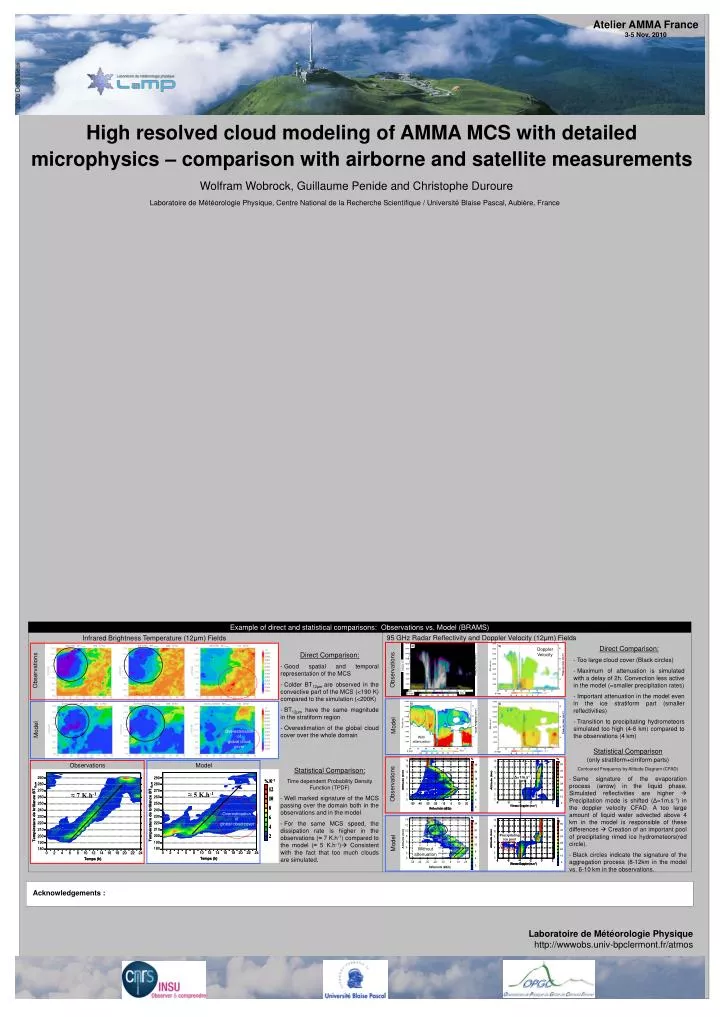
Example of direct and statistical comparisons: Observations vs. Model (BRAMS) Reflectivity Doppler Velocity Observations Observations Observations Model Model Overestimation of global cloud cover Model Δ=1m.s-1 Observations ≈ 5 K.h-1 ≈ 7 K.h-1 Overestimation of global cloud cover Precipitating ice pool Model Atelier AMMA France 3-5 Nov. 2010 High resolved cloud modeling of AMMA MCS with detailed microphysics – comparison with airborne and satellite measurements Wolfram Wobrock, Guillaume Penide and Christophe Duroure Laboratoire de Météorologie Physique, Centre National de la Recherche Scientifique / Université Blaise Pascal, Aubière, France 95 GHz Radar Reflectivity and Doppler Velocity (12μm) Fields Infrared Brightness Temperature (12μm) Fields • Direct Comparison: • Too large cloud cover (Black circles) • Maximum of attenuation is simulated with a delay of 2h. Convection less active in the model (=smaller precipitation rates) • Important attenuation in the model even in the ice stratiform part (smaller reflectivities) • Transition to precipitating hydrometeors simulated too high (4-6 km) compared to the observations (4 km) • Direct Comparison: • Good spatial and temporal representation of the MCS • Colder BT12μm are observed in the convective part of the MCS (<190 K) compared to the simulation (<200K) • BT12μm have the same magnitude in the stratiform region • Overestimation of the global cloud cover over the whole domain With attenuation • Statistical Comparison • (only stratiform+cirriform parts) • Contoured Frequency by Altitude Diagram (CFAD) • Same signature of the evaporation process (arrow) in the liquid phase. Simulated reflectivities are higher Precipitation mode is shifted (Δ=1m.s-1) in the doppler velocity CFAD. A too large amount of liquid water advected above 4 km in the model is responsible of these differences Creation of an important pool of precipitating rimed ice hydrometeors(red circle). • Black circles indicate the signature of the aggregation process (8-12km in the model vs. 6-10 km in the observations. • Statistical Comparison: • Time dependent Probability Density Function (TPDF) • Well marked signature of the MCS passing over the domain both in the observations and in the model • For the same MCS speed, the dissipation rate is higher in the observations (≈ 7 K.h-1) compared to the model (≈ 5 K.h-1) Consistent with the fact that too much clouds are simulated. Without attenuation Time (h) Time (h) Acknowledgements : Laboratoire de Météorologie Physique http://wwwobs.univ-bpclermont.fr/atmos