Download
1 / 47
470 likes | 473 Views
Scoring Rules, Generalized Entropy, and Utility Maximization. Victor Jose, Robert Nau, & Robert Winkler Fuqua School of Business Duke University. Presentation for GRID/ENSAM Seminar Paris, May 22, 2007. Overview.

E N D
Scoring Rules, Generalized Entropy, and Utility Maximization Victor Jose, Robert Nau, & Robert Winkler Fuqua School of Business Duke University Presentation for GRID/ENSAM Seminar Paris, May 22, 2007
Overview • Scoring rules are reward functions for defining subjective probabilities and eliciting them in forecasting applications and experimental economics (de Finetti, Brier, Savage, Selten...) • Cross-entropy, or divergence, is a physical measure of information gain in communication theory and machine learning (Shannon, Kullback-Leibler...) • Utility maximization is the decision maker’s objective in Bayesian decision theory and game theory (von Neumann & Morgenstern, Savage...)
General connections • Any decision problem under uncertainty may be used to define a scoring rule or measure of divergence between probability distributions. • The expected score or divergence is merely the expected-utility gain that results from solving the problem using the decision maker’s “true” (or posterior) probability distribution p rather than some other “baseline” (or prior) distribution q. • These connections have been of interest in the recent literature of robust Bayesian inference and mathematical finance.
Specific results • We explore the connections among the best-known parametric families of generalized scoring rules, divergence measures, and utility functions. • The expected scores obtained by truthful probability assessors turn out to correspond exactly to well-knowngeneralized divergences. • They also correspond exactly to expected-utility gains in financial investment problems with utility functions from the linear-risk-tolerance (a.k.a. HARA) family. • These results generalize to incomplete markets via a primal-dual pair of convex programs.
Part 1: Scoring rules • Consider a probability forecast for a discrete event with npossible outcomes (“states of the world”). • Let ei = (0, ..., 1, ..., 0) denote the indicator vector for the ith state (where 1 appears in the ith position). • Let p = (p1, ..., pn) denote the forecaster’s true subjective probability distribution over states. • Let r = (r1, ..., rn) denote the forecaster’s reported distribution(if different from p). (Later, let q = (q1, ..., qn) denote a baseline distribution upon which the forecaster seeks to improve.)
Definition of a scoring rule • A scoring rule is a function S(r, p)that determines the forecaster’s score (reward) for reporting r when her true distribution is p. • The actual score is S(r, ei) when the ith state occurs. • S(p) S(p, p) will denote the forecaster’s expected score for truthfully reporting her true distribution p
Proper scoring rules • The scoring rule S is [strictly] proper if S(p) [>] S(r, p) for all r [p], i.e., if the forecaster’s expected score is [uniquely] maximized when she reports her true probabilities. • S is [strictly] proper iff S(p) is a [strictly] convex function of p. • If S is strictly proper, then it is uniquely determined from S(p) by McCarthy’s (1956) formula: S(r, p) = S(r) + S(r)· (p r)
Standard scoring rules The three most commonly used scoring rules are: • The quadratic scoring rule: S(p, ei ) = (ei p2)2 • The spherical scoring rule: S(p, ei ) = pi /p2 • The logarithmic scoring rule: S(p, ei ) = ln( pi )
History of common scoring rules • The quadratic scoring rule was introduced by de Finetti (1937, 1974) to define subjective probability; later used by Brier (1950) as a tool for evaluating and paying weather forecasters; also used to reward subjects in economic experiments. • Selten (1998) has presented an axiomatic argument in favor of the quadratic rule. • The spherical and logarithmic rules were introduced by I.J. Good (1971), who also noted that the spherical and quadratic rules could be generalized to positive exponents other than 2, leading to...
Generalized scoring rules • Power scoring rule ( quadratic at = 2): • Pseudospherical scoring rule ( spherical at = 2) • Both rules rescaled logarithmic rule at = 1. • Under both rules, the payoff profile (risk profile) is an affine function of pi1
“Baseline” distribution? • The standard scoring rules are symmetric across states: • Payoffs in different states are ranked in order of pi • The optimal expected score is minimized whenp is the uniform distribution • Hence these rules implicitly reward the forecaster for departures from a uniform distribution • But is the uniform distribution the appropriate “baseline” against which to measure the value of a forecast?
Rationale for a non-uniform baseline • In nearly all applications outside of laboratory experiments, the relevant baseline is not uniform: • Weather forecasting • Economic forecasting • Technological forecasting • Demand for new products • Financial markets • Sports betting • We therefore propose that the score be should be “weighted” by a non-uniform baseline distribution q s.t. the optimal expected score is minized at p = q
How should the dependence on a baseline distribution be modeled? • We propose that the scoring rule should rank payoffs in order of pi/qi, i.e., the relative, not absolute, value of piin comparison with qi. • Rationales for this form of dependence: • A $1 bet on state i at odds determined by qihas an expected payoff of pi/qi, hence relative probabilities are what matter for purposes of betting. • Payoffs ought not to depend on the outcomes of statistically independent events that have the same probabilities under p and q, and this also constrains the payoffs to depend on the ratio pi/qi .
Weighted scoring rules • The power and pseudospherical rules can be weighted by an arbitrary baseline distribution q merely by replacing pi1 with (pi /qi)1 in the formulas that determine the profiles of payoffs. • They can also be normalized so as to be valid for all real and to yield a score of zero in all states iff p q, so that the expected score is positive iff p q. • The weighted rules thus measure the “information value” of knowing that the distribution is p rather than qas seen from the forecaster’s perspective.
With this weighting and normalization, the power and pseudospherical rules become: • The weightedpower scoring rule: • The weighted pseudospherical scoring rule:
Properties of weighted scoring rules • Both rules are strictly proper for all real. • Both rules weighted logarithmic ruleln(pi/qi) at =1. • For the same p,q, and , the vector of weighted power scores is an affine transformation of the vector of weighted pseudospherical scores, since both are affine functions of (pi/qi)1. • However, the two rules present different incentives for information-gathering and honest reporting. • The special cases = 0 and = ½ have interesting properties but have not been previously studied.
Special cases of weighted scores Power Pseudospherical
Weighted expected score functions • Weighted power expected score: • Weighted pseudospherical expected score:
Behavior of the weighted power score for n = 3. • For fixed p and q, the scores diverge as . • For << 0 [ >> 2] only the lowest [highest] probability event is distinguished from the others.
By comparison, the weighted pseudospherical scores approach fixed limits as . • Again, for << 0 [ >> 2] only the lowest [highest] probability event is distinguished from the others.
The corresponding expected scores vs. are equal at = 1, where both rules converge to the weighted logarithmic scoring rule, but elsewhere the weighted power expected score is strictly larger.
Part 2. Entropy • In statistical physics, the entropy of a system with n possible internal states having probability distribution p is defined (up to a multiplicative constant) by • In communication theory, the negative entropy H(p) is the “self-information” of an event from a stationary random process with distribution p, measured in terms of the average number of bits required to optimally encode it (Shannon 1948).
The KL divergence • The cross-entropy, or Kullback-Leibler divergence, between two distributions p and q measures the expected information gain (reduction in average number of bits per event) due to replacing the “wrong” distribution q with the “right” distribution p:
Properties of the KL divergence • Additivity with respect to independent partitions of the state space: • Thus, if A and B are independent events whose initial distributions qA and qBare respectively updated to pA and pB, the total expected information gain in their product space is the sum of the separate expected information gains, as measured by their KL divergences.
Properties of the KL divergence • Recursivity with respect to the splitting of events: • Thus, the total expected information gain does not depend on whether the true state is resolved all at once or via a sequential splitting of events.
Other divergence/distance measures • The Chi-square divergence (Pearson 1900) is used by frequentist statisticians to measure goodness of fit: • The Hellinger distance is a symmetric measure of distance between two distributions that is popular in machine learning applications:
Onward to generalized divergence... • The properties of additivity and recursivity can be considered as axioms for a measure of expected information gain which imply the KL divergence. • However, weaker axioms of “pseudoadditivity” and “pseudorecursitivity” lead to parametric families of generalized divergence. • These generalized divergences “interpolate” and “extrapolate” beyond the KL divergence, the Chi-square divergence, and the Hellinger distance.
Power divergence • The directed divergence of order , a.k.a. the power divergence, was proposed by Havrda & Chavrát (1967) and elaborated by Rathie & Kannappan (1972), Cressie & Read (1980), Haussler and Opper (1997): • It is pseudoadditive and pseudorecursive for all , and it coincides with the KL divergence at = 1. • It is the weighted power expected score, hence: The power divergence is the implicit information measure behind the weighted power scoring rule.
Pseudospherical divergence • An alternative generalized entropy was introduced by Arimoto (1971) and further studied by Sharma & Mittal (1975), Boekee & Van der Lubbe (1980) and Lavenda & Dunning-Davies (2003), for >1: • The corresponding divergence, which we call the pseudospherical divergence, is obtained by introducing a baseline distribution q and dividing out the unnecessary in the numerator:
Properties of the pseudospherical divergence • It is defined for all real (not merely > 1). • It is pseudoadditive but generally not pseudorecursive. • It is identical to the weighted pseudospherical expected score, hence: The pseudospherical divergence is the implicit information measure behind the weighted pseudospherical scoring rule.
Interesting special cases • The power and pseudospherical divergences both coincide with the KL divergence at = 1. • At = 0, = ½, and = 2 they are linearly (or at least monotonically) related to the reverse KL divergence, the squared Hellinger distance, and the Chi-square divergence, respectively:
Where we’ve gotten so far... • There are two parametric families of weighted, strictly proper scoring rules which correspond exactly to two well-known parametric families of generalized divergence, each of which has a full “spectrum” of possibilities ( < < ). • But what is the decision-theoretic significance of these quantities? • What are some guidelines for choosing among the the two families and their parameters?
Part 3. Decisions under uncertainty with linear risk tolerance • Suppose a decision maker with subjective probability distribution p and utility function u bets or trades optimally against a risk-neutral opponent or contingent claim market with distribution q. • For any risk-averse utility function, the investor’s gain in expected utility yields an economic measure of the divergence between pand q. • In particular, suppose the investor’s utility function belongs to the linear risk tolerance (HARA) family, i.e., the family of generalized exponential, logarithmic, and power utility functions.
Two canonical decision problems: • Problem “S”: A risk averse decision maker with probability distribution p and utility function u(x) for time-1 consumption bets optimally at time 0 against a risk-neutral opponent with distribution q to obtain the expected utility: Feasibility constraint:x must have non-negative expected value for opponent Decision maker’s payoff vector Decision maker’s expected utility
Two canonical problems, continued: • Problem “P”: A risk averse decision maker with distribution p and quasilinear utility function a + u(b), where a is time-0 consumption and b is time-1 consumption, bets optimally at time 0 against a risk-neutral opponent with distribution q, to obtain the expected utility: Utility lost at time 0 (cost of x) Expected utility gained at time 1 Decision maker’s time-1 payoff vector
Risk aversion and risk tolerance • Let x denote gain or loss relative to a (riskless) status quo wealth position, and let u(x) denote the utility of x. • The monetary quantity (x) u (x)/u (x) is the investor’s local risk tolerance at x(the reciprocal of the Pratt-Arrow measure of local risk aversion). • The usual decision-analytic rule of thumb is as follows: an investor who has received y and has local risk tolerance (x) is roughly indifferent to accepting a50-50 gamble between the wealth positions x (x) and x ½(x), i.e., indifferent to gaining (x) or losing ½(x) with equal probability.
Linear risk tolerance (LRT) utility • The most commonly used utility functions in decision analysis and financial economics have the property of linear risk tolerance, i.e., (x) = + x,where > 0is the risk tolerance coefficient. • W.l.o.g. the units of money and utility can be scaled so that u(0) = 0 and u (0) = 1, and (x) = 1 + x, so that marginal utility and risk tolerance are equal to 1 at x = 0, and the LRT utility function has the form:
Special cases of normalized LRT utility Note the symmetry around = ½...
Qualitative properties of LRT utility The graphs of u(x) and u1 (x), whose powers are reciprocal to each other, are symmetric around the line y = x. Reciprocal Reciprocal Exponential Log Quadratic Square root Power Power1/ ...where = (1)/
Extension to imprecise probabilities/incomplete markets • Suppose the decision maker faces a risk neutral opponent with imprecise probabilities (or an incomplete market) whose beliefs (prices) determine only a convex set Q of probability distributions. • Then the utility-maximization problems S and P generalize into convex programs whose duals are the minimization of the corresponding divergences (expected scores).
Generalization of problem S • A payoff vector xis feasible for the decision maker if the opponent’s (market’s) payoff –x has non-negative expectation for every q in Q. • Primal problem: Find x in nto maximize Ep[u(x)] subject to Eq[x] 0 for all q in Q. • Dual problem: Find q in Q that minimizes , the pseudospherical divergence from p.
p q Q Generalization of problem S: p = precise probability of a risk averse decision maker with utility function u Q = set of imprecise probabilities of risk neutral opponent/market Finding the payoff vector x to maximize Ep[u(x)] s.t. Eq[x] 0 is equivalent (dual) to finding q in Q to minimize the divergence S(pq)
Generalization of problem P • A time-1 payoff vector xcan be purchased for a price w at time 0 if the opponent’s (market’s) payoff –x has an expected value of at least w for every q in Q • Primal problem: Find x in nto maximize Ep[u(x)] w subject to Eq[x]w for all q in Q. • Dual problem: Find q in Q that minimizes , the power divergence from p.
Conclusions • The power & pseudospherical scoring rules can (and should) be generalized by incorporating a not-necessarily-uniform baseline distribution. • The resulting weighted expected scores are equal to well-known generalized divergences, with KL divergence as the special case = 1. • These scoring rules and divergences also arise as the solutions to utility maximization problems with LRT utility in 1 period or quasilinear LRT utility in 2 periods, where the baseline distribution describes the beliefs of a risk neutral betting opponent (or market)
Conclusions • When the baseline distribution is imprecise (market incompleteness), the problem of maximizing expected utility is the dual of the problem of minimizing the corresponding divergence. • These results shed more light on the connection between utility theory and information theory, particularly with respect to commonly-used parametric forms of utility and divergence. • For the weighted power and pseudospherical scoring rules, values of between 0 and 1 appear to be the most interesting, and the cases = 0 and = ½ have been so far under-explored.
Conclusions • The power & pseudospherical scoring rules can be improved by incorporating a not-necessarily-uniform baseline distribution. • The resulting weighted expected scores are equal to well-known generalized divergences (with KL divergence as the special case = 1) • These scoring rules and divergences also arise as the solutions to utility maximization problems with LRT utility in 1 period or quasilinear LRT utility in 2 periods. • Values of between 0 and 1 appear to be the most interesting, and the cases = 0 and = ½ have been so far under-explored.