Solving Differential Equations using MATLAB: Notes on using dsolve ('eqn1','eqn2', ...)

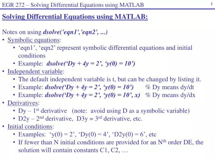
1. EGR 272 – Solving Differential Equations using MATLAB • Solving Differential Equations using MATLAB: • Notes on using dsolve('eqn1','eqn2', ...) • Symbolic equations: • ‘eqn1’, ‘eqn2’ represent symbolic differential equations and initial conditions • Example: dsolve(‘Dy + 4y = 2’, ‘y(0) = 10’) • Independent variable: • The default independent variable is t, but can be changed by listing it. • Example: dsolve(‘Dy + 4y = 2’, ‘y(0) = 10’) % Dy means dy/dt • Example: dsolve(‘Dy + 4y = 2’, ‘y(0) = 10’, x) % Dy means dy/dx • Derivatives: • Dy – 1st derivative (note: avoid using D as a symbolic variable) • D2y – 2nd derivative, D3y = 3rd derivative, etc. • Initial conditions: • Examples: ‘y(0) = 2’, ‘Dy(0) = 4’, ‘D2y(0) = 6’, etc • If fewer than N initial conditions are provided for an Nth order DE, the solution will contain constants C1, C2, …

2. EGR 272 – Solving Differential Equations using MATLAB Example: Solve for y(t) in the following first-order DE if y(0) = 8 MATLAB Solution:

3. EGR 272 – Solving Differential Equations using MATLAB Example: Solve for y(t) in the following second-order DE if y(0) = 2 and y’(0) = -4 MATLAB Solution: Note: This example uses a forcing function of 10e-2t (right-side of the equation). In EGR 270 we will only deal with DC sources, so the forcing functions will always be constants.

4. EGR 272 – Solving Differential Equations using MATLAB Graphing the Solution to a Differential Equation: Since the solution to a differential equation is a symbolic equation, it can easily be graphed using ezplot. Example: Graph the solution to the previous example: Discussion: Does this graph satisfy the initial and final values for v(t)?

5. EGR 272 – Solving Differential Equations using MATLAB Class Example:A) Solve for v(t) in the following 1st- order DEif v(0) = 12 B) Repeat this example using MATLAB Graph the solution using ezplot( ) from 0 to 5

6. EGR 272 – Solving Differential Equations using MATLAB Class Example:A) Solve for i(t) in the following 2nd-order DE if i(0) = 6, i’(0) = 38 B) Repeat this example using MATLAB Graph the solution using ezplot( ) from 0 to 5

7. EGR 272 – Solving Differential Equations using MATLAB • Significance of overdamped, critically damped, and underdamped solutions • A circuit with an overdamped response is called an overdamped circuit (similar for the other types of damping). What does this mean about the circuit? • First, some definitions: • Damping – the act of removing oscillations • Example: A shock absorber might be adjusted so that it doesn’t oscillate, but smoothly returns a wheel to its initial position after an impact. • Example: A switch is thrown in a circuit and an output voltage adjusts to a new level. • In an overdamped circuit, it would reach the new level smoothly and without oscillation (ringing). • In an underdamped circuit, it would oscillate as it approached the new level. • See the illustration on the following slide.

8. EGR 272 – Solving Differential Equations using MATLAB Example: Different types of damping in an RLC circuit For the circuit below we can easily see that v(0) = 0V and v() = 10V. So when the switch closes at t = 0, how does v(t) get to 10V? This is a 2nd-order circuit, so it must have a 2nd-order response. So it must be overdamped, underdamped, or critically damped. Sketch v(t) below. v(t) t

9. EGR 272 – Solving Differential Equations using MATLAB Example: The DE for v(t) in the circuit below if L = 100 H and C = 10 uFis: A) What value of R results in a critically-damped circuit? • Use MATLAB so solve the DE and graph the response for: • R = 200 (critically damped) • R = 350 (overdamped) • R = 50 (underdamped)

10. EGR 272 – Solving Differential Equations using MATLAB Example: (continued) Solve and graph the DE for R = 350, 200, and 50 using MATLAB.