Download
1 / 24
240 likes | 250 Views
Modelling advection with MOHID. Contents. What is advection? The importance of advection in coastal areas Methodology implemented in MOHID to simulate advection Code trip; Test cases 1D and 2 D cyclic channel; Symetric estuary Freshwater cylinder Density front. What is advection ?. k.

E N D
Contents • What is advection? • The importance of advection in coastal areas • Methodology implemented in MOHID to simulate advection • Code trip; • Test cases • 1D and 2 D cyclic channel; • Symetric estuary • Freshwater cylinder • Density front
What is advection ? k i j
The importance of advection in coastal waters • Estuary mouths – horizontal advection of momentum; • Coastal Upwelling – vertical and horizontal advection of heat; • Baroclinic instabilities – horizontal advection of mass, of heat and of momentum;
Upwelling in schematic coast Schematic slope
Upwelling scenario – more important because is the scenario more common in summer
Density front Ajustamento geostrófico segundo um modelo analítico baseado nas equações de gravidade reduzida a) Instante inicial (velocidade perpendicular à frente); b) instante em que é atingido o equilíbrio velocidade paralela à frente.
Baroclinic instability • Vorticidade potencial (explicação de oceanógrafo) w (f+w)/H= const. H H w • Balanço de forças (explicação de engenheiro)
Methodology implemented in Mohid to compute advection Central Differences 2nd order upwind (1D Quick) 3th order upwind (1D Quickest)
Problems related with higher order schemes Ok Vi Vi-1>>Vi Or Vi-1<<Vi Problems =0 Vi-1
Problems related with higher order schemes Lack of positivity – production of ripples near sharp gradients
Total Variation Diminishing • TVD schemes implemented in Mohid • if r>0 • MinMod : =min(1,r) • Van Leer : =2r/(1+r) • MUSCL : min(2,2r,(1+r)/2) • SuperBee : max(min(1,2r),min(r, 2)) • PPM :max(min(Aux,2/(1-Cr),2r/Cr)) • a = 0.5 + (1 - 2.*abs(cr))/6 • b = 0.5 - (1 - 2.*abs(cr))/6 • Aux = a + b * r • Else • =0 • endif A value for function of the spatial variability of P is compute in a way that the problems describe in the earlier slide r<0=> =0 in all schemes r>0
Code Trip • The nuclear subroutine is ComputeAdvectionFace: • The advective flux in each face can depend of the property value in the follow compute points (i-2, i-1, I, i+1) • This subroutine compute for each face the coefficients a, b, c and d
Test cases • Already tested • 1D and 2 D cyclic channel; • Symetric estuary • Need more testing • Fresh water cylinder • Density front
Fresh Water Cylinder - Exercise • Depth = 20 m, 20 layers • 30 km x 30 km, dx = 1 km • Latitude 52º N • Cylinder of 10 m deep and 3 km of radius. Outside the cylinder salinity is 34.85 psu Within the cylinder the salinity and the density variability is given by: • Run period 144 h • Bottom rugosity =0 • Null turbulent diffusion or minimal values to avoid instabilities • A relaxation boundary condition for the water level and salinity. Relax in the boundary the water level to 0 and salinity to 34.85 psu. A four-point-wide relaxation zone:
Conclusions • The TVD with a Superbee limitation looks to be so far the best method. However, in extreme cases it generates wiggles;
Future Work • Introduce the cross-derivates in the Quick and Quickest methods.
Bibliography • Pietrzak, J. (1997). The use of TVD limiters for forward-in-time upstream-biased advection schemes in ocean modeling. Monthly Weather Review. Volume 126, 812-830, 1997 . • Burchard, H., and K. Bolding, GETM - a general estuarine transport model. Scientific documentation, Tech. Rep. EUR 20253 EN, European Commission, 2002. • James I.D. (1996). "Advection schemes for shelf sea models." Journal of Marine Systems 8: 237-254. • James, I. D. (2000). "A high-performance explicit vertical advection scheme for ocean models: how PPM can beat the CFL condition." Applied Mathematical Modelling, 24(1): 1-9. • Tartinville, B., E. Deleersnijder, P. Lazure, R. Proctor, K.G. Ruddick and R.E. Uittenbogaard (1998). "A coastal ocean model intercomparison study for a three-dimensional idealised test case." Applied Mathematical Modelling, 22(3): 165-182. • Shchepetkin, A., & J.C. McWilliams, 1998: Quasi-monotone advection schemes based on explicit locally adaptive dissipation. Monthly Weather Review, 126, 1541-1580.