Download
1 / 52
520 likes | 528 Views
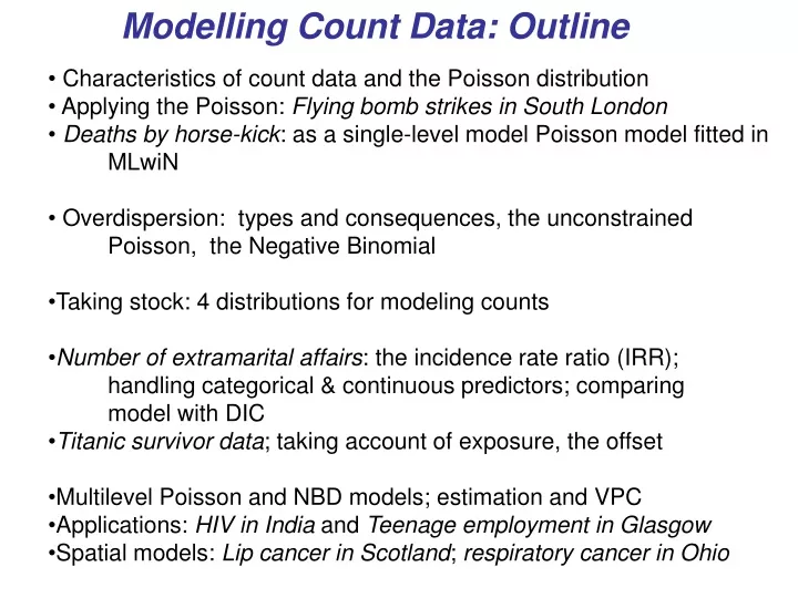
Modelling Count Data: Outline. Characteristics of count data and the Poisson distribution Applying the Poisson: Flying bomb strikes in South London Deaths by horse-kick : as a single-level model Poisson model fitted in MLwiN

E N D
Modelling Count Data: Outline • Characteristics of count data and the Poisson distribution • Applying the Poisson: Flying bomb strikes in South London • Deaths by horse-kick: as a single-level model Poisson model fitted in MLwiN • Overdispersion: types and consequences, the unconstrained Poisson, the Negative Binomial • Taking stock: 4 distributions for modeling counts • Number of extramarital affairs: the incidence rate ratio (IRR); handling categorical & continuous predictors; comparing model with DIC • Titanic survivor data; taking account of exposure, the offset • Multilevel Poisson and NBD models; estimation and VPC • Applications: HIV in India and Teenage employment in Glasgow • Spatial models: Lip cancer in Scotland; respiratory cancer in Ohio
Some characteristics of count data • Very common in the social sciences • Number of children; Number of marriages • Number of arrests; Number of traffic accidents • Number of flows; Number of deaths • Counts have particular characteristics • Integers & cannot be negative • Often positively skewed; a ‘floor’ of zero • In practice often rare events which peak at 1,2 or 3 and rare at higher values • Modelled by • Logit regression models the log odds of an underlying propensity of an outcome; • Poisson regression models the log of the underlying rateof occurrence of a count.
Theoretical Poisson distribution I • The Poisson distribution results if the underlying number of random events per unit time or space have a constant mean ()rate of occurrence, and each event is independent Simeon-Denis Poisson (1838) Research on the Probability of Judgments in Criminal and Civil Matters • Applying the Poisson: Flying bomb strikes in South London • Key research question: falling at random or under a guidance system • If random independent events should be distributed spatially as a Poisson distribution • Divide south London into 576 equally sized small areas (0.24km2) • Count the number of bombs in each area and compare to a Poisson • Mean rate = = [229(0) + 211(1) + 93(2) + 35(3) + 7(4) +1(5)]/576 • = 0.929 hits per unit square • Very close fit; concluded random
Theoretical Poisson distribution II Probability mass function(PMF) for 3 different mean occurrences • When mean =1; very positively skewed • As mean occurrence increases (more common event), distribution approaches Gaussian; • So use Poisson for ‘rareish’ events; mean below 10 • Fundamental property of the Poisson: mean = variance • Simulated 10,000 observations according to Poisson • Mean Variance Skewness • 0.993 0.98 1.00 • 4.001 4.07 0.50 • 10.03 10.38 0.33 • Variance is not a freely estimated parameter as in Gaussian
Death by Horse-kick I: the data • Bortkewicz L von.(1898) The Law of Small Numbers, Leipzig • No of soldiers killed annually by horse-kicks in Prussian cavalry; 10 corps over 20 years (occurrences per unit time) • The full data 200 corps years of observations • As a frequency distribution (grouped data) • Deaths 0 1 2 3 4 5+ • Frequency 109 65 22 3 1 0 Mean Variance Number of obs • 0.61 0.611 200 • Interpretation: mean rate of 0.61 deaths per cohort year (ie rare) • Mean equals variance, therefore a Poisson distribution
Death by Horse-kick II: as a Poisson Again :The Poisson results if underlying number of random events per unit time or space have a constant mean () rate of occurrence, and each event is independent • With a mean (and therefore a variance) of 0.61 • Deaths 0 1 2 3 4 5+ • Frequency 109 65 22 3 1 0 • Theory 109 66 20 4 1 1 • Formula for Poisson PMF • e is base of the natural logarithm (2.7182) • is the mean (shape parameter): the average number of events in a given time interval • x! is the factorial of x EG: mean rate of 0.6 accidents per corps year; what is probability of getting 3 accidents in a corps in a year?
Horse-kick III: as a single level Poisson model General form of the single-level model Observed count is distributed as an underlying Poisson with a mean rate of occurrence of ; That is as an underlying mean and level-1 random term of z0 (the Poisson ‘weight’) Mean rate is related to predictors non-linearly as an exponential relationship Model loge to get a linear model (log link) The Poisson weight is the square root of estimated underlying count, re-estimated at each iteration Variance of level-1 residuals constrained to 1, • Modeling on the loge scale, cannot make prediction of a negative count on the raw scale • Level-1 variance is constrained to be an exact Poisson, (variance =mean)
Horse-kick IV: Null single-level Poisson model in MLwiN • The raw ungrouped counts are modeled with a log link and a variance constrained to be equal to the mean • -0.494 is the mean rate of occurrence on the log scale • Exponentiate -0.494 to get the mean rate of 0.61 • 0.61 is interpreted as RATE; the number of events per unit time (or space), ie 0.61 horse-kick deaths per corps-year
Overdispersion I: Types and consequences • So far; equi-dispersion, variances equal to the mean • Overdispersion: variance > mean; long tail, eg LOS (common) • Un-dispersion: variance < mean; data more alike than pure Poisson process; in multilevel possibility of missing level • Consequences of overdispersion • Fixed part SE’s "point estimates are accurate but they are not as precise as you think they are" • In multilevel, mis-estimate higher-level random part • Apparent and true overdispersion: thought experiment • : number of extra-marital affairs: men women with different means • apparent: mis-specified fixed part, not separated out distributions with different means • true: genuine stochastic property of more inherent variability • in practice model fixed part as well as possible, and allow for overdisperion
Overdispersion II: the unconstrained Poisson • Deaths by horse-kick • estimate an over- dispersed Poisson • allow the level-1 variance to be estimated • Not significantly different from 1; • No evidence that this is not a Poisson distribution
Overdispersion III: the Negative binomial • Instead of fitting an overdispersed Poisson, could fit a NBD model • Handles long-tailed distributions; • An explicit model in which variance is greater than the mean • Can even have an over-dispersed NBD • Same log-link but NBD has 2 parameters for the level-1 variance; that is quadratic level-1 variance, v is the overdispersion parameter
Overdispersion IV: the Negative binomial • Horse=kick analysis: • Null single-level NBD model; essentially no change, v is estimated to be 0.00 (see with Stored model; Compared stored model) • Overdispersed negative binomial; • No evidence of overdispersion; deaths are independent
Linking the Binomial and the Poisson: I • First Bernoulli and Binomial • Bernoulli is a distribution for binary discrete events • y is observed outcome; ie 1 or 0 • E(y) = ; underlying propensity/probability for occurrence • Var(y) = /1- • Binomial is a distribution for discrete events out of a number of trials • y is observed outcome; n is the number of trials, • E(y) = ; underlying propensity/ of occurrence • Var(y) = [/(1- )]/n • Least variation when denominator is large (more reliable), and as underlying probability approaches 0 or 1
Linking the Binomial and the Poisson: II • Poisson is limit of a binomial process in which prob → 0, n→∞ • Poisson describes the probability that a random event will occur in a time or space interval when the probability is very small, the number of trials is very large, and each event is independent • EG : The probability that any automobile is involved in an accident is very small, but there are very many cars on a road in a day so that the distribution (if each crash is independent) follows a Poisson count • If non-independence of crashes (a ‘pile-up’), then over-dispersed Poisson/NBD, latter used for ‘contagious’ processes • In practice, Poisson and NBD used for rare occurrences, less than 10 cases per interval,& hundreds or even thousands for denominator/ trials [Clayton & Hills (1993)Statistical Models in Epidemiology OUP]
Taking stock: 4 distributions for counts • If common rate of occurrence (mean >10) then use raw counts and Gaussian distribution (assess Normality assumption of the residuals) • If rare rate of occurrence, then use over-dispersed Poisson or NBD; the level-1 unconstrained variance estimate will allow assessment of departure from equi-dispersion; improved SE’s, but biased estimates if apparent overdispersion due to model mis-specification • Use the Binomial distribution if count is out of some total and the event is not rare; that is numerator and denominator of the same order • Mean variance relations for 4 different distributions that could be used for counts
Modeling number of extra-marital affairs Single- level Poisson with Single categorical Predictor Extract of raw data (601 individuals from Fair 1978) Fair, R C(1978) A theory of extramarital affairs, Journal of Political Economy, 86(1), 45-61 • Single categorical predictor Children with NoKids, as the base • Understanding customized predictions…………….
Single- level Poisson with Single categorical Predictor Understanding customized predictions • Log scale: • NoKids: -0.092 WithKids-0.092+0.606= 0.514 • First use equation to get underyling log-number of events then exponeniate to get estimated count (since married) • As mean/median counts • NoKids: expo(-0.092)= 0.91211 • Withkids: expo(-0.092 + 0.606) = 1.6720 • Those with children have a higher average rate of affairs (but have they been married longer?)
Modeling number of extra marital affairs: the incidence rate ratio (IRR) So far: mean counts NoKids: expo(-0.092)= 0.91211 Withkids: expo(-0.092 + 0.606) = 1.6720 But also as IRR; comparing the ratio of those with and without kids IRR = 1.6720/0.91211 = 1.8331 That is Withkids have a 83% higher rate BUT can get this directly from the model by exponentiating the estimate for the contrasted category expo(0.606) = 1.8331 • Rules: • exponeniating the estimates for the (constant plus the contrasted category) gives the mean rate for the contrasted category • b) ) exponeniating the contrasted category gives IRR in comparison to base category
Why is the exponentiated coefficient a IRR? • As always, the estimated coefficient is the change in response corresponding to a one unit change in the predictor • Response is underlying logged count • When Xi is 0 (Nokids); log count| Xi is 0 = β0 • But when Xi is 1(Withkids); log count| Xi is 1 = β0 + β1 X1i • Subtracting the first equation from the second gives • (log count| Xi is 1)-(log count| Xi is 0) = β1 • Exponentiating both sides gives (note the division sign) • (count| Xi is 1)/(count| Xi is 0) = exp(β1) • Thus, exp(β1) is a rate ratio corresponding to the ratio of the mean number of affairs for a with-child person to the mean number of affairs without-child person • Incidence: number of new cases • Rate: because it number of events per time or space • Ratio: because its is ratio of two rates
Modeling number of extra-marital affairs: changing the base category • Previously contrasted category: Withkids: +0.606 • Now contrasted category: Nokids : -0.606 • Changing base simply produces a change of sign on the loge scale • Exponentiating the contrasted category: • Before: expo(+0.606) = 1.8331 • Now: expo(-0.606) = 0.5455 • Doubling the rate on loge scale is 0.693; Halving the rate on loge scale is -0.693 • IRR of 0.111 = IRR of 9-fold increase, difficult to appreciate • Advice: choose base category to be have the lowest mean rate; get positive contrasted estimates; always then comparing a larger value to a base of 1
Affairs: modeling a set of categorical predictors • A model with ‘years married’ included with < 4 years as base Customised predictions: mean rate, IRR, & graph with 95% CI’s
Affairs: modeling a continuous predictor Age Age as a 2nd order polynomial centred around 17 years (the youngest person in survey; also lowest rate • To get mean rate as it changes with age • Expo (-0.990 + 0.149*(Age-17) -0.003*(Age-17)2) • To get IRR in comparison for a person aged 33 compared to 17 • Expo( 0.149*16) –(0.003 *162) (drop the constant!) • Easiest interpreted as graphs!
Affairs: a SET of predictors & models • Notice substantial overdispersion • Poisson & extra-Poisson no change in estimates; some change to NBD • Notice larger SE’s when allow for overdispersion; NBD most conservative • In full model, WithKids not significant
NBD model for Marital Affairs • IRR of 1 for Under 4 years married, Very religious, No children, aged 17 • Previous Age effect is really length of marriage • Used comparable vertical axes, range of 4
NBD model for number of Extra-Marital Affairs • With 95% confidence intervals • NB that they are asymmetric on the unlogged scale
Affairs: Evaluating a sequence of models using DIC • Likelihood and hence the Deviance are not available for Poisson and NBD models fitted by quasi-likelihood • DIC criterion available though MCMC; typically needs larger number of iterations than Normal & Binomial (suggested default is 50k not 5k) • Currently MCMC not available in MLwiN for over-dispersed Poisson nor NBD models; so have to use Wald tests in Intervals and tests window
Titanic survivor data: Taking account of exposure • So far, response is observed count, now we want to model a count given exposure: EG only 1 high-class female child survived but only 1 exposed! Here 2 possible measures of exposure a) the number of potential cases; could use a binomial b) the expected number if everyone had the same exposure (i indexes cell) Death rate = Total Deaths/ Total exposed =817/1316 = 0.379179 Expi = Casesi * Survival rate Latter often used to treat the exposure as a nuisance parameter & allows calculation of Standardised Rate’s SRi = Obsi/Expi * 100 Previous examples Horsekick: Exposure removed by design: 200 cohort years Affairs: included length of marriage; theoretically interesting
Modeling SR’s: the use of the OFFSET Model: SRi = (Obsi/Expi) = F(Agei, Genderi, Classi) Where i is a cell, groups with same characteristics Aim: are observed survivors greater or less than expected, and how these ‘differences’ are related to a set of predictor variables? As a non-linear model: E(SRi)= E(Obsi/Expi) = As a linear model (division of raw data is subtraction of a log) Loge (Obsi) - Loge(Expi)) = As a model with an offset, moving Loge(Expi) to the right-hand side, and constraining coefficient to be 1; ie Exp becomes predictor variable Loge (Obsi) = 1.0* Loge(Expi) + NB MLwiN automatically loge transforms the observed response; you have to create the loge of the expected and declare it as an offset Sir John Nelder
Surviving on the Titanic as a log-linear model • Include the offset • As a saturated model; ie Age *Gender*Class, (2*2*3), 12 terms for 12 cells • Make predictions on the loge scale (must include constant); exponentiate all terms to get departures from the expected rate, that is modeled SR’s
Titanic survival: parsimonious model • Remove insignificant terms starting with 3-way interactions for High*women*children Customized predictions: Very low rates of survival for Low and Middle class adult men; large gender gap for adults, but not for children
Titanic survival: parsimonious model • Modeled SR’s and descriptive SR’s • Ordered by worse survival • Estimated SR’s only shown if 95% CI’s do not include 1.0
Two-level multilevel Poisson One new term, the level 2 differential, on the loge scale, is assumed to come from Normal distribution with a variance of • Can also fit Poisson multilevel with offset and NBD multilevel in MLwiN
Estimation of multilevel Poisson and NBD in MLwiN I • Same options as for binary and binomial • Quasi-likelihood and therefore MQL or PQL fitted using IGLS/RIGLS; fast, but no deviance (have to use Wald tests); may be troubled by small number of higher-level units; simulations have shown that MQL tends to overestimate the higher-level variance parameters • MCMC estimates; good quality and can use DIC to compare Poisson models; but currently MCMC is not possible for extra-Poisson nor for NBD • MCMC in MLwiN often produces highly correlated chains (in part due to the fact that the parameters of the model are highly correlated; variance =mean) Therefore requires substantial number of simulations; typically much larger than for Normal or for Binomial
Estimation of multilevel Poisson and NBD in MLwiN II • Possibility to output to WinBUGS and use the univariate AR sampler and Gamerman (1997) method which tends to have less correlated chains, but WinBUGS is considerably slower generally [Gamerman, D. (1997) Sampling from the posterior distribution in generalized linear mixed models. Statistics and Computing 7, 57-68] • Advice: start with IGLS PQL; switch to MCMC, be prepared to make 500,000 simulations (suggest use 1 in 10 thinning to store the chains); use Effective sample size to assess required length of change, eg need ESS of at least 500 for key parameters of interest; compare results and contemplate using PQL and over-dispersed Poisson • Freely available software MIXPREG for multilevel Poisson counts including offsets; uses full information maximum likelihood estimated using quadrature http://tigger.uic.edu/~hedeker/mixpcm.PDF
VPC for Poisson models • Can either use • Simulation method to derive VPC (modify the binomial procedure) • Use exact method: http://people.upei.ca/hstryhn/iccpoisson.ppt (Henrik Stryhn) • VPC for two level random intercepts model (available for other models) Clearly VPC depends on and
Modeling Counts in MLwiN: HIV in India Aim: investigate the State geography of HIV in terms of riskData: nationally representative sample of 100k individuals in 2005- 2006Response: HIV sero-status from blood samplesStructure: 1720 cells within 28 States; cells are a group of people who share common characteristics [Age-Groups(4), Education(4), Sex(2), Urbanity(2) and State (28)]Rarity: only 467 sero-positives were foundModel: Log count of number of seropositives in a cell related to an offset of Log expected count if national rates appliedPredictors of Age, Sex and Education and UrbanityTwo-level multilevel Poisson, extra-Poisson & NBD
HIV in India: Standardized Morbidity Rates Higher educated females have the lowest risk, across the age-groups
HIV in India: some results Risks for different States relative to living in urban and rural areas nationally.
Modeling proportions as a binomial in MLwiN • exactly the same procedure as for binary models • except that observed y is a proportion (not just 1 and 0, the denominator (n) is variable (not just 1) and extra-dispersion at level 1 is allowed (not just exact binomial) • Reading: • Subramanian S V, Duncan C, Jones K (2001) Multilevel perspectives on modeling census data Environment and Planning A33(3) 399 – 417
Data: teenage employment In Glasgow districts • “Ungrouped” data that is individual data • Model binary outcome of employed or not and two individual predictors
Same data as a multilevel structure: a set of tables for each district GENDER QUALIF MALE FEMALE Postcode UnErate LOW 5 out of 6 3 out of 12 G1A 15% HIGH 2 out of 7 7 out of 9 LOW 5 out of 9 7 out of 11 G1B 12% HIGH 8 out of 8 7 out of 9 LOW 3 out of 3 - G99Z 3% HIGH 2 out of3 out of 5 • Level 1 cell in table • Level 2: Postcode sector • Margins: define the two categorical predictors • Internal cells: the response of 5 out of 6 are employed
Teenage unemployment: some results from a binomial, two-level logit model
A B Person in A Affected by A(SH) and B,C,D (MM) C D E F Person in H Affected by H(SH) and E,I,K,G (MM) G H I J K L M Multiple membership defined by common boundary; weights as function of inverse distance between centroids of areas Spatial Models as a combination of strict hierarchy and multiple membership: counts are commonly used
Scottish Lip Cancer Spatial multiple-membership model • Response: observed counts of male lip cancer for the 56 regions of Scotland (1975-1980) • Predictor: % of workforce working in outdoor occupations (Agric;For; Fish) Expected count based on population size • Structure areas and their neighbours defined as having a common border (up to 11); equal weights for each neighbouring region that sum to 1 • Rate of lip cancer in each region is affected by both the region itself and its nearest neighbours after taking account of outdoor activity • Model Log of the response related to fixed predictor, with an offset, Poisson distribution for counts; • NB Two sets of random effects • 1 area random effects; (ie unstructured; non-spatial variation); • 2 multiple membership set of random effects for the neighbours of each region
MCMC estimation: 50,000 draws Poisson model Fixed effects: Offset and Well-supported + relation Well-supported Residual neighbourhood effect NB: Poisson highly correlated chains
Scottish Lip Cancer: CAR model CAR: CAR one set of random effects, which have an expected value of the average of the surrounding random effects; weights divided by the number of neighbours where ni is the number of neighbours for area i and the weights are typically all 1 • MLwiN: limited capabilities for CAR model; ie at one level only (unlike Bugs)
MCMC estimation: CAR model, 50,000 draws Poisson model Fixed effects: Offset and Well-supported + relation Well-supported Residual neighbourhood effect
Ohio cancer: repeated measures (space and time!) • Response: counts of respiratory cancer deaths in Ohio counties • Aim: Are there hotspot counties with distinctive trends? (small numbers so ‘borrow strength’ from neighbours) • Structure: annual repeated measures (1979-1988) for counties • Classification 3: n’hoods as MM (3-8 n’hoods) • Classification 2: counties (88) • Classification 1: occasion (88*10) • Predictor: Expected deaths; Time • Model Log of the response related to fixed predictor, with an offset, Poisson distribution for counts (C1); • Two sets of random effects • 1 area random effects allowed to vary over time; trend for each county from the Ohio distribution (c2) • 2 multiple membership set of random effects for the neighbours of each region (C3)
MCMC estimation: repeated measures model, 50,000 draws General trend N’hood variance Variance function for between county time trend Default priors