POMDPs

1. POMDPs Slides based on Hansen et. Al.’s tutorial + R&N 3rd Ed Sec 17.4

2. Planning using Partially Observable Markov Decision Processes: A Tutorial Presenters: Eric Hansen, Mississippi State University Daniel Bernstein, University of Massachusetts/Amherst Zhengzhu Feng, University of Massachusetts/Amherst Rong Zhou, Mississippi State University

3. Introduction and foundations Definition of POMDP Goals, rewards and optimality criteria Examples and applications Computational complexity Belief states and Bayesian conditioning

4. Planning under partial observability Imperfect observation Goal Environment Environment Action

5. Two Approaches to Planning under Partial Observability • Nondeterministic planning • Uncertainty is represented by set of possible states • No possibility is considered more likely than any other • Probabilistic (decision-theoretic) planning • Uncertainty is represented by probability distribution over possible states • In this tutorial we consider the second, more general approach

6. Markov models

7. Definition of POMDP s0 S2 S1 hidden states: z2 z0 z1 observations: a2 actions: a0 a1 rewards: r0 r2 r1

8. Goals, rewards and optimality criteria • Rewards are additive and time-separable, and objective is to maximize expected total reward • Traditional planning goals can be encoded in reward function Example: achieving a state satisfying property P at minimal cost is encoded by making any state satisfying P a zero-reward absorbing state, and assigning all other states negative reward. • POMDP allows partial satisfaction of goals and tradeoffs among competing goals • Planning horizon can be finite, infinite or indefinite

9. Machine Maintenance X Canonical application of POMDPs in Operations Research

10. +1 –1 Start 0.1 0.8 0.1 Robot Navigation • Canonical application of POMDPs in AI • Toy example from Russell & Norvig’s AI textbook Actions: N, S, E, W, Stop Observations: sense surrounding walls

11. Many other applications • Helicopter control [Bagnell & Schneider 2001] • Dialogue management [Roy, Pineau & Thrun 2000] • Preference elicitation [Boutilier 2002] • Optimal search and sensor scheduling [Krishnamurthy & Singh 2000] • Medical diagnosis and treatment [Hauskrecht & Fraser 2000] • Packet scheduling in computer networks [Chang et al. 2000; Bent & Van Hentenryck 2004]

12. Computational complexity • Finite-horizon • PSPACE-hard [Papadimitriou & Tsitsiklis 1987] • NP-complete if unobservable • Infinite-horizon • Undecidable [Madani, Hanks & Condon 1999] • NP-hard for -approximation [Lusena, Goldsmith & Mundhenk 2001] • NP-hard for memoryless or bounded-memory control problem [Littman 1994; Meuleau et al. 1999]

13. POMDP • <S, A, T, R, Ω, O> tuple • S, A, T, R of MDP • Ω – finite set of observations • O:SxA-> Π(Ω) • Belief state • - information state • – b, probability distribution over S • - b(s1)

14. POMDP • Goal is to maximize expected long-term reward from the initial state distribution • State is not directly observed a world o

15. Two sources of POMDP complexity • Curse of dimensionality • size of state space • shared by other planning problems • Curse of memory • size of value function (number of vectors) • or equivalently, size of controller (memory) • unique to POMDPs dimensionality memory Complexity of each iteration of DP:

16. Two representations of policy • Policy maps history to action • Since history grows exponentially with horizon, it needs to be summarized, especially in infinite-horizon case • Two ways to summarize history • belief state • finite-state automaton – partitions history into finite number of “states”

17. Belief simplex S2 S1 (0, 0, 1) (0, 1) 0 S0 0 (1, 0) S1 (0, 1, 0) (1, 0, 0) S0 2 states 3 states

18. a1 z1 z2 z1 z2 a2 P(s0) = 0 P(s0) = 1 Belief state has Markov property • The process of maintaining the belief state is Markovian • For any belief state, the successor belief state depends only on the action and observation

19. Belief-state MDP • State space: the belief simplex • Actions: same as before • State transition function: P(b’|b,a) = e E P(b’|b,a,e)P(e|b,a) • Reward function: r(b,a) =sS b(s)r(s,a) • Bellman optimality equation: Should be Integration…

20. P(b|b,a,e) Current Belief State (Register) Policy  e b a b Obs. Action Belief-state controller “State Estimation” • Update belief state after action and observation • Policy maps belief state to action • Policy is found by solving the belief-state MDP

21. POMDP as MDP in Belief Space

22. Dynamic Programming for POMDPs • We’ll start with some important concepts: a1 o1 o2 a2 a3 o1 o2 o1 o2 a3 a2 a1 a1 s1 s2 belief state policy tree linear value function

23. Dynamic Programming for POMDPs a1 a2 s1 s2

24. a1 a2 a1 a2 a2 a1 a2 a1 o1 o1 o2 o2 o1 o1 o1 o1 o1 o1 o2 o2 o2 o2 o2 o2 a1 a1 a1 a1 a1 a1 a2 a2 a2 a2 a1 a1 a2 a2 a2 a2 Dynamic Programming for POMDPs s1 s2

25. a1 a2 a1 a2 o1 o1 o2 o2 o1 o1 o2 o2 a1 a1 a1 a1 a2 a1 a2 a2 Dynamic Programming for POMDPs s1 s2

26. Dynamic Programming for POMDPs s1 s2

27. [Finitie Horizon Case] POMDP Value Iteration: Basic Idea

28. First Problem Solved • Key insight: value function • piecewise linear & convex (PWLC) • Convexity makes intuitive sense • Middle of belief space – high entropy, can’t select actions appropriately, less long-term reward • Near corners of simplex – low entropy, take actions more likely to be appropriate for current world state, gain more reward • Each line (hyperplane) represented with vector • Coefficients of line (hyperplane) • e.g. V(b) = c1 x b(s1) + c2 x (1-b(s1)) • To find value function at b, find vector with largest dot pdt with b

29. POMDP Value Iteration: Phase 1: One action plans Two states: 0 and 1 R(0)=0 ; R(1) = 1 [stay]0.9 stay; 0.1 go [go] 0.9 go; 0.1 stay Sensor reports correct state with 0.6 prob Discount facto=1

30. stay 0 1 stay stay POMDP Value Iteration: Phase 2: Two action (conditional) plans

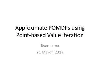
32. Point-based Value Iteration: Approximating with Exemplar Belief States

33. Solving infinite-horizon POMDPs • Value iteration: iteration of dynamic programming operator computes value function that is arbitrarily close to optimal • Optimal value function is not necessarily piecewise linear, since optimal control may require infinite memory • But in many cases, as Sondik (1978) and Kaelbling et al (1998) noticed, value iteration converges to a finite set of vectors. In these cases, an optimal policy is equivalent to a finite-state controller.

34. q2 q1 q2 o1 o2 o1 s1q1 s1q2 o2 o1 o2 o2 o1 s2q1 s2q2 o2 o1 Policy evaluation As in the fully observable case, policy evaluation involves solving a system of linear equations. There is one unknown (and one equation) for each pair of system state and controller node

35. z0,z1 2 a0 z0,z1 0 a0 z0,z1 0 a0 0 a0 z0,z1 z0 z0 3 a1 z0 3 a1 z0,z1 z0 z1 z1 1 a1 4 a0 1 a1 z0,z1 4 a0 z1 z1 V(b) V(b) V(b) 0,2 0 0 3 3 4 4 1 1 0 1 0 1 0 1 Policy improvement

36. Per-Iteration Complexity of POMDP value iteration.. Number of a vectors needed at tth iteration Time for computing each a vector

37. Approximating POMDP value function with bounds • It is possible to get approximate value functions for POMDP in two ways • Over constrain it to be a NOMDP: You get Blind Value function which ignores the observation • A “conformant” policy • For infinite horizon, it will be same action always! (only |A| policies) • Relax it to be a FOMDP: You assume that the state is fully observable. • A “state-based” policy Under-estimates value (over-estimates cost) Over-estimates value (under-estimates cost) Per iteration

38. Upper bounds for leaf nodes can come from FOMDP VI and lower bounds from NOMDP VI Observations are written as o or z

39. Comparing POMDPs with Non-deterministic conditional planning POMDP Non-Deterministic Case

40. RTDP-Bel doesn’t do look ahead, and also stores the current estimate of value function (see update)

41. ---Slides BeyonD This Not Covered--

42. Two Problems • How to represent value function over continuous belief space? • How to update value function Vt with Vt-1? • POMDP -> MDP S => B, set of belief states A => same T => τ(b,a,b’) R => ρ(b, a)

43. Running Example • POMDP with • Two states (s1 and s2) • Two actions (a1 and a2) • Three observations (z1, z2, z3) 1D belief space for a 2 state POMDP Probability that state is s1

44. Second Problem • Can’t iterate over all belief states (infinite) for value-iteration but… • Given vectors representing Vt-1, generate vectors representing Vt

45. Horizon 1 • No future • Value function consists only of immediate reward • e.g. • R(s1, a1) = 0, R(s2, a1) = 1.5, • R(s1, a2) = 1, R(s2, a2) = 0 • b = <0.25, 0.75> • Value of doing a1 • = 1 x b(s1) + 0 x b(s2) • = 1 x 0.25 + 0 x 0.75 • Value of doing a2 • = 0 x b(s1) + 1.5 x b(s2) • = 0 x 0.25 + 1.5 x 0.75

46. Second Problem • Break problem down into 3 steps • -Compute value of belief state given action and observation • -Compute value of belief state given action • -Compute value of belief state

47. Horizon 2 – Given action & obs • If in belief state b,what is the best value of • doing action a1 and seeing z1? • Best value = best value of immediate action + best value of next action • Best value of immediate action = horizon 1 value function

48. Horizon 2 – Given action & obs • Assume best immediate action is a1 and obs is z1 • What’s the best action for b’ that results from initial b when perform a1 and observe z1? • Not feasible – do this for all belief states (infinite)

49. Horizon 2 – Given action & obs • Construct function over entire (initial) belief space • from horizon 1 value function • with belief transformation built in

50. Horizon 2 – Given action & obs • S(a1, z1) corresponds to paper’s • S() built in: • - horizon 1 value function • - belief transformation • - “Weight” of seeing z after performing a • - Discount factor • - Immediate Reward • S() PWLC