An introduction to Ultraviolet/Visible Absorption Spectroscopy

1. An introduction to Ultraviolet/Visible Absorption Spectroscopy Lectures 21 and 22

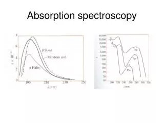
2. In this chapter: Absorption by molecules, rather than atoms, is considered. • Absorption in the UV and Vis regions: occurs due to electronic transitions from the ground state to excited state. • Broad band spectra are obtained: Because molecules have vibrational and rotational energy levels associated with electronic energy levels. • The signal is either absorbance or percent transmittance of the analyte solution where:

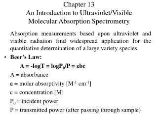
3. Absorption measurements based upon ultraviolet and visible radiation: Find widespread application for the quantitative determination of a large variety species. Beer’s Law: A = -logT = logP0/P = bc Where T = P/Po always a fraction) A = absorbance = molar absorptivity [M-1 cm-1] c = concentration [M] P0= incident power P = transmitted power (after passing through sample) b= path length in cm

4. Example: A solution containing 4.48 ppm KMnO, had a % transmittance of 30.9% in a 1.00 cm cell at 520 nm. Calculate the molar ahsorptivity of KMnO4, at 520 nm. A = εbc mmol KMnO4/mL = (4.48 mg KMnO4/1000 mL) x (mmol KMnO4/158 mg KMnO4) = 2.84x10-5 M T = 0.309 A = - log T = - log 0.309 = 0.510 0.510 = ε * 1.00 cm * 2.84x10-5 mol/L ε = 1.80x104 L mol-1 cm-1

7. Some losses of radiation power P Po Loses about 8.5 % of incident radiation from reflections

8. Measurement of Transmittance and Absorbance: The power of the beam transmitted by the analyte solution is usually compared with the power of the beam transmitted by an identical cell containing only solvent or blank (zero abs). An experimental transmittance and absorbance are then obtained with the equations. = - log T = log1/T P0 and P: refers to the power of radiation after it has passed through the solvent and the analyte. Because T is a fraction so generally multiplied by 100 to give %T

9. Beer’s law and mixtures Each analyte present in the solution absorbs light! The magnitude of the absorption depends on its e A total = A1+A2+…+An A total = e1bc1+e2bc2+…+enbcn If e1 = e2 =en then simultaneous determination is impossible (difficult to separate conc. of substances. seam to be same substance). Need to measure A at nl’s(get n2e’s) to solve for the concentration of species in the mixture For 3 substance we need to measure at 9 e Where  is max for each substance

10. b=1cm Large slope = large e and good sensitivity

11. Limitations to Beer’s Law Deviation from linearity of the A and C relationship (remember no interpolation and extrapolation of the calibration: It is regions of deviation from linearity) Types of deviations: • Real limitations (present in the law itself) • Chemical deviations • Instrumental deviations

12. 1.      Real Limitations a. Beer’s law is good for dilute analyte solutions only. • High concentrations (> 0.01M) will cause a negative error since as the distance between molecules become smaller; the charge distribution will be affected which alter the molecules ability to absorb a specific wavelength. • The same phenomenon is also observed for solutions with high electrolyte concentration, even at low analyte concentration. Both give –ve effect • The molar absorptivity is altered due to electrostatic interactions.

13. b. (e) depends on refractive index. • The refractive index is a function of concentration. • Therefore, e will be concentration dependent. • However, the refractive index changes very slightly for dilutesolutions and thus we can practically assume that e is constant. c. In rare cases, the molar absorptivity changes widely with concentration, even at dilute solutions. • Therefore, Beer’s law is never a linear relation for such compounds, like methylene blue.

14. 2.  Chemical Deviations: This factor is an important one which largely affects linearity in Beer’s law. It originates when an analyte1) dissociates, 2) associates, or 3) reacts in the solvent, or one of matrix constituents. For example: An acid base indicator when dissolved in water will partially dissociate according to its acid dissociation constant:

15. HIn(color 1)  H+ + In- (color 2) It can be easily appreciated that the amount of HIn present in solution is less than that originally dissolved where: CHIn [HIn] + [In-] Assume an analytical concentration of 2x10-5 M indicator (ka = 1.42x10-5) was used, we may write:

16. 1.42x10-5 = x2/(2x10-5 – x) Solving the quadratic equation gives: X = 1.12x10-5 M which means: [In-] = 1.12x10-5 M [HIn] = 2x10-5 – 1.12x10-5 = 0.88x10-5 M Therefore, the absorbance measured will be the sum of that for HIn and In-. If a 1.00 cm cell was used and the e for both HIn and In- were 7.12x103 and 9.61x102 Lmol-1cm-1at 570 nm, respectively, the absorbance of the solution can be calculated:

17. A = AHIn + AIn A = 7.12x103 * 1.00* 0.88x10-5 + 9.61x102 * 1.00 *1.12x10-5 = 0.073 However, if no dissociation takes place we may have: A = AHIn (Theoretically) A = 7.12x103 * 1.00 * 2x10-5 = 0.142 If the two results are compared we can calculate the % decrease in anticipated signal as: % decrease in signal = {(0.142 – 0.073)/0.142}x100% = 49% As a result of dissociation

18. However, at 430 nm, the molar absorptivities of HIn and In- are 6.30*102 and 2.06*104, respectively. A = AHIn + AIn A = 6.30*102 * 1.00* 0.88x10-5 + 2.06*104 * 1.00 *1.12x10-5 = 0.236 Again, if no dissociation takes place we may have: A = AHIn(Theoretically) A = 6.30*102 * 1.00 * 2x10-5 = 0.013 If the two results are compared we can calculate the % increase in anticipated signal as: % increase in signal = {(0.236 – 0.013)/0.013}x100% = V. large Error as a result of dissociation

19. Comparison between results obtained at 570 nm and 430 nm show large dependence on the values of the molar absorptivities of HIn and In- at these wavelength. At 570 nm: A = AHIn + AIn A = 7.12x103 * 1.00* 0.88x10-5 + 9.61x102 * 1.00 *1.12x10-5 = 0.073 And at 430 nm: A = 6.30*102 * 1.00* 0.88x10-5 + 2.06*104 * 1.00 *1.12x10-5 = 0.236

20. Chemical deviations from Beer’s law for unbuffered solutions of the indicator Hln. Note that there are: • positive deviations at 430 nm • negative deviations at 570 nm. At 430 nm: The absorbance is primarily due to the ionized In-form of the indicator and is proportional to the fraction ionized, which varies nonlinearly with the total indicator concentration. At 570 nm: The absorbance is due principally to the undissociated acid Hln, which increases nonlinearly with the total concentration.

21. +ve error -ve error

22. Calculated Absorbance Data for Various Indicator Concentrations

23. An example of association equilibria: Association of chromate in acidic solution to form the dichromate according to the equation below: 2 CrO42- + 2 H+D Cr2O72- + H2O The absorbance of the chromate ions will change according to the mentioned equilibrium and will thus be nonlinearly related to concentration. A = eCrO4 *b*CCrO4 + eCr2O7 *b*CCr2O7 If the two e are equals no error

24. 3.   Instrumental Deviations. a. Beer’s law is good for monochromatic light only since e is wavelength dependent. • It is enough to assume a dichromatic beam passing through a sample to appreciate the need for a monochromatic light. • Assume that the radiant power of incident radiation is Po and Po’ while transmitted power is P and P’. • The absorbance ( at two ) of solution can be written as:

25. A = log (Po + Po’)/(P + P’) at the two  P = Po10-ebc, (from the log Eq.) substituting in the above equation: A = log (Po + Po’)/(Po10-ebc Po’10-e’bc)for diff. e Assume e = e’ = e A = log (Po + Po’)/(Po + Po’) 10-ebc A = ebc However, since e’ # e, since e is wavelength dependent, then A # ebc not a linear relationship between abs. and c Result: Beers law is good for monochromatic radiation. But for different lamps or polych. there is a deviation

27. The effect of polychromatic radiation on Beer’s law. • In the spectrum at the left, the molar absorptivity of the analyte is nearly constant over band A. • Note that in Beer’s law plot at the right, using band A gives a linear relationship. • In the spectrum, band B corresponds to a region where the absorptivity shows substantial changes. • In the lower plot, note the dramatic deviation from Beer’s law that results.

28. Sign. change in e (diff. abs.) No sign. change in e same abs.

29. Therefore, the linearity between absorbance and concentration breaks down if incident radiation was polychromatic. • In most cases with UV-Vis spectroscopy, the effect is small especially at the wavelength maximum. • The small changes in signal is insignificant since e differs only slightly.

30. UV-Vis Absorption Spectroscopy Lecture 23

31. b.  Stray Radiation أشعة ضالة Stray radiation resulting from scattering or various reflections in the instrument will reach the detector without passing through the sample. • The problem can be severe in cases of: 1- High absorbance. 2- When the wavelengths of stray radiation is in such a range where the detector is highly sensitive as well as at wavelengths extremes of an instrument. • The absorbance recorded can be represented by the relation: A = log (Po + Ps)/(P + Ps) Solvent sample Error due to Ps: Ps is added not multiplied Where; Ps is the radiant power of stray radiation.

33. Instrumental Noise as a Function in Transmittance The uncertainty in concentration as a function of the uncertainty in transmittance can be statistically represented as: sc2 = (dc/dT)2 sT2 sTisuncertainty of transmitance A = -log T = ebc = -0.434 ln T c = -(1/eb)*0.434 ln T (1) dc/dT = - 0.434/ebT sc2 = (-0.434/ebT)2 sT2 (2)

34. Dividing equation 2 by the square of equation 1 (sc/c)2 = (-0.434/ebT)2 sT2/{(-0.434 ln T)2/(eb)2} sc/c = (sT / T ln T) •  Therefore, it is clear that the uncertainty in concentration of a sample is nonlinearly related to the magnitude of the transmittance. • Substitution for different values of transmittance and assuming sT is constant, we get:

36. Very lower unc. in con at : Abs: 0.2-0.7

37. Therefore, an absorbance between 0.2-0.7 may be advantageous in terms of a lower uncertainty in concentration measurements. • At higher or lower absorbances, an increase in uncertainty is encountered. • It is therefore advised that the test solution be in the concentration range which gives an absorbance value in the range from 0.2-0.7 for best precision. • However, it should also be remembered that we ended up with this conclusion provided that sT is constant. • Unfortunately, sT is not always constant which complicates the conclusions above.

38. EFFECT OF bandwidth which is related to slit width Effect of bandwidth on spectral detail for a sample of benzene vapor. Note that as the spectral bandwidth increases, the fine structure in the spectrum is lost. At a bandwidth of 10 nm, only a broad absorption band is observed.

39. Effect of slit width (spectral bandwidth) on peak heights. Here, the sample was a solution of praseodymium chloride. Note that as the spectral bandwidth decreases by decreasing the slit width from 1.0 mm to 0.1 mm, the peak heights increase. لتحسين الاشارة يتم التضييق تدريجيا للحصول على أحسن امتصاص اي ثبات للاشارة قبل النزول

40. Effect of Scattered Radiation at Wavelength Extremes of an Instrument Wavelength extremes of an instrument are dependent on: • Type of source • Type of detector • Type of optical components used in the manufacture of the instrument. Outside the working range of the instrument: It is not possible to use it for accurate determinations (at extremes unc. increases). However, the extremes of the instrument are very close to the region of invalid instrumental performance and would thus be not very accurate.

41. An example: A visible photometer which, in principle, can be used in the range from 340-780 nm. It may be obvious that glass windows, cells and prism will start to absorb significantly below 380 nm and thus a decrease in the incident radiant power is significant.

42. What defines the instrumental wavelength extremes? Three main Factors: • Source • Detector • Optical components (lenses, windows, etc) Measurements at wavelength extremes should be avoided since errors are very possible due to: • Source limitations • Detector limitations • Sample cell limitations • Scattered radiation

43. B: UV-VIS spectrophotometer A: VIS spectrophotometer EFFECT OF SCATTERED RADIATION Spectrum of cerium (IV) obtained with a spectrophotometer having glass optics (A) and quartz optics (B). The false peak in A arises from transmission of stray radiation of longer wavelengths.

44. The output from the source at the low wavelength range is minimal. • Also, the detector has best sensitivities around 550 nm which means that away up and down this value, the sensitivity significantly decrease. • However, scattered radiation, and stray radiation in general, will reach the detector without passing through these surfaces as well as these radiation are constituted from wavelengths for which the detector is highly sensitive. • In some cases, stray and scattered radiation reaching the detector can be far more intense than the monochromatic beam from the source. • False peaks may appear in such cases and one should be aware of this cause of such peaks.

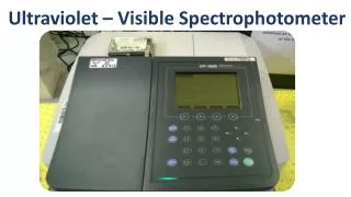
45. (Abs. Inst.)Instrumentation • Light source •  - selector • Sample container • Detector • Signal processing Light Sources (commercial instruments) • D2 lamp (UV: 160 – 375 nm) • W lamp (vis: 350 – 2500 nm)

46. Sources (UV)1) Deuterium and hydrogen lamps (160 – 375 nm) D2 + Ee→ D2* → D’ + D’’ + h

47. Deuterium lamp UV region (a) A deuterium lamp of the type used in spectrophotometers and (b) its spectrum. The plot is of irradiance Eλ (proportional to radiant power) versus wavelength. Note that the maximum intensity occurs at ~225 m. Typically: Instruments switch from deuterium to tungsten at ~350 nm.

48. 2) Tungsten lamp: Visible and near-IR region • A tungsten lamp of the type used in spectroscopy and its spectrum. (b) Intensity of the tungsten source is usually quite low at wavelengths shorter than about 350 nm. Note that the intensity reaches a maximum in the near-IR region of the spectrum.

49. The tungsten lamp is by far the most common source in the visible and near IR region with a continuum output wavelength in the range from 350-2500 nm. • The lamp is formed from a tungsten filament heated to about 3000 oC housed in a glass envelope. • The output of the lamp approaches a black body radiation where it is observed that the energy of a tungsten lamp varies as the fourth power of the operating voltage.

50. Tungsten halogen lamps are currently more popular than just tungsten lamps since they have longer lifetime. • Tungsten halogen lamps contain small quantities of iodine in a quartz envelope. • The quartz envelope is necessary due to the higher temperature of the tungsten halogen lamps (3500 oC). • The longer lifetime of tungsten halogen lamps stems from the fact that sublimed tungsten forms volatile WI2 which redeposits on the filament thus increasing its lifetime. • The output of tungsten halogen lamps are more efficient and extend well into the UV.