Inspection- “back-end quality control”

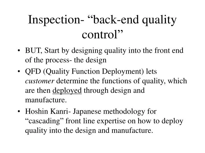
1. Inspection- “back-end quality control” • BUT, Start by designing quality into the front end of the process- the design • QFD (Quality Function Deployment) lets customer determine the functions of quality, which are then deployed through design and manufacture. • Hoshin Kanri- Japanese methodology for “cascading” front line expertise on how to deploy quality into the design and manufacture.

2. Inspection Costs Total Cost Cost of inspection Cost of passing defectives Optimal

3. Using SPC as part of the inspection process • “Is our process in control?” • I.e. what are the limits we set, using statistics to determine if we need to take corrective action • process distribution vs. sample distribution • We use a sampling distribution of means of measurements… because it is normal and has less variability. (we’re taking averages of averages) • even though the process distribution may not be normal, stats theory tells us the distribution of samples means probably is • Translated: We take numerous samples of numerous observations

4. Samplingdistribution Processdistribution Mean A sample of means has less variability because the data has been “smoothed” twice

5. Setting control limits • We usually use 2 standard deviations from mean (about 95% of distribution captured) or 3 standard deviations from mean (about 99.7% captured) to set control limits • Any values that fall outside of these limits are considered “out of control”… and usually are considered non-random, and therefore, actionable variations • TYPE I error: sample mean falls outside of control limits when variation is actually random • TYPE II: mean inside control limits when actually non-random

6. /2 /2 Mean LCL UCL Probabilityof Type I error Type I Error

7. Abnormal variationdue to assignable sources Out ofcontrol UCL Mean Normal variationdue to chance LCL Abnormal variationdue to assignable sources 0 1 2 3 4 5 6 7 8 9 10 11 12 13 14 15 Sample number Control Chart

8. Calculating Control limits for variables- mean charts • Monitor how close the data sticks to the average when we are measuring (not counting) • Control Limits= the average of sample means + & - (z * sample means ) • Z is determined by how much of the distribution you want to consider “in control” (Usually 2 or 3) • sample means=std dev. of process samples/ square root of the number of samples

9. Calculating mean chart control limits

10. What happens when we go to z=2?

11. Range charts- a different perspective • While mean charts are sensitive to changes in the process mean, range charts give you a feel for process dispersion • Because mean charts take averages of means, they don’t tell you when variability is increasing in the process

12. Does notreveal increase x-Chart UCL Mean and Range Charts Sampling Distribution (process variability is increasing) R-chart Reveals increase

13. Control charts for summarizing attributes of process, e.g. defects • Used when variables are counted, not measured • P-chart monitors proportion of defectives • used in binomial distribution situations (e.g. answer is “good” or “bad” • p= proportion of defectives • UCL = p + z(p ) • LCL = p - z(p ) • p = SQR RT of(p(1-p)/n) where n= sample size of each observation

14. P-chart example. Are we in control?

15. C-charts: use when non-occurrences can’t be counted (i.e. a continuous variable) • Example: initial defects per units of new cars • Control limits = c + & - z*(SQR RT of c) • where c= mean # of defects per unit • and std dev = SQR RT of (c)

16. You try one • What is mean defects per unit? • 116.25 • What is Square root of c? • 10.78 • What’s the limits @ z=2? • 116+ 2*10.78=137.56 • 116-2*10.78=94.44 • In control? • NO

17. c-chart example. You do z=3.

18. Run tests • Sometimes, all data within a control chart may be within limits, but there is a trend or cycle to the data within limits. This trend or cycle may need management action. • Example: machine tolerances loosen before weekend down time, within limits. • Run tests attempt to characterize these trends or cycles.

19. Process Capability analysis • Comparing process variability with designed- for variability. (“Are we producing our Mercedes only to Yugo tolerances?” • Expressed in terms of standard deviation • typically +&- 3 standard deviations from mean (total of 6) “6 sigma quality”

20. Let’s do one • Given that machine tolerance is defined as .75mm-1.25mm and you get to choose from 3 machines, which can you choose? • Therefore, width= .50 mm (1.25-.75) • Machine (mm) (given) Capability • A .05 • B .08 • C .12

21. Let’s do one • Given that machine tolerance is defined as .75mm-1.25mm and you get to choose from 3 machines • Machine (mm) (given) Capability • A .05 .05*6=.30 • B .08 .08*6=.48 • C .12 .12*6=.72 • MACHINES A & B function within the .50 specification (1.25-.75).

22. Now compute the capability ratio • Given that machine tolerance is defined as .75mm-1.25mm and you get to choose from 3 machines • Process capability ratio Cp= specification width (“what is our tolerance”)/ process width of machine • same as saying upper spec-lower spec/ 6 of machine • Machine (mm) (given) Cp • A .05 .50/.30=1.66 • B .08 .50/.48=1.04 • C .12 .50/.72=0.69 • MACHINE A is preferable because it has the highest capability ratio. It has the greatest probability of functioning within design specs. • Any machine with ratio >= 1.33 is acceptable in generally accepted practiced

23. For next time • Chapter 10 PROBLEMS 2,3,6 to hand in • For problem 3, pay special attention to range chart factors in the body of the chapter • For problem 2, use appropriate Z table from back of book.

25. Problem 2 A) mean = 1 ; std. dev = 0.1 n=25 observations z=2.17 (to get 97%) Control limits are mean + and - z*(std dev./ square root of n) (see page 448) UCL = 1+ 2.17*(.01/SQR(25))= 1.004 LCL = 1 – 2.17* (.01/SQR(25))= 0.996 The 5th sample mean of 0.995 is out of control, and should be investigated. See page 881. We’re using this chart because we’re analyzing both “tails” for upper and lower control limits. Because this table only shows area from mean to one tail, you look for the Z value equal to .9700/2.

26. Problem 3 we don’t know the std dev. of process sample First get your mean of X and mean of R. Mean of x= 18.6/6=3.1, Mean of R (range) = 2.7/6= .45 Range chart factors table in body of the chapter gives you factors to plug into a formula if you want to compute range chart UCL and LCL figures to 3S if std deviation of process sample is unknown. Let's do the range chart first. The formulas given are UCL = D4*(mean of R) and LCL = D3*(mean of R) In this problem, you are told that n=20. So, start by pulling all the info off table 10-2 you see: at n=20... A2= 0.18; D3=0.41; and D4= 1.59. Now, you need to figure out your control limits. UCL = D4* mean of R = 1.59*.45=.7155 LCL = D3* mean of R = .41 * .45 =.1845 Now let's do mean chart control limits. From page 470, your mean chart limit formulas using sample range are: UCL = mean of x + A2*R =3.1+ (.18*.45) = 3.181 LCL = mean of x - A2*R = 3.1 - (.18*.45) = 3.019 Now, you can compare x and r values from the data to see if they are within limits.

27. Problem 6 • “must be repeated” is code for binomials, and therefore proportion. So, use formulas for p-chart. • Given n=200; z =2 • In sample 1, p= 1/200= .005 • the mean of p= 25/(13*200)= .0096 • Control limits = .0096 + & - 2* SQR((mean of p* 1- mean of p)/n)= .0096 + & - .0138 • = .0234 and -.0042 (effectively 0)

28. Problem 6 continued • Now, as instructed, we’ll throw out sample 10 (it’s value is too large) and re-compute • mean of p= 18/(12*200) = .0075 • Limits = .0075 + & - = .0197 and = -.005 (0)