Download
1 / 38
380 likes | 385 Views
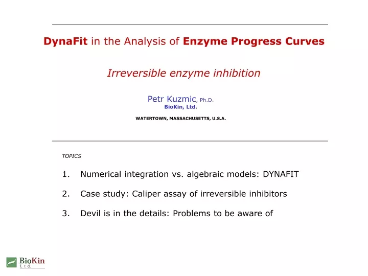
DynaFit in the Analysis of Enzyme Progress Curves Irreversible enzyme inhibition. Petr Kuzmic , Ph.D. BioKin, Ltd. WATERTOWN, MASSACHUSETTS, U.S.A. TOPICS Numerical integration vs. algebraic models: DYNAFIT Case study: Caliper assay of irreversible inhibitors

E N D
DynaFit in the Analysis of EnzymeProgress CurvesIrreversible enzyme inhibition Petr Kuzmic, Ph.D.BioKin, Ltd. WATERTOWN, MASSACHUSETTS, U.S.A. • TOPICS • Numerical integration vs. algebraic models: DYNAFIT • Case study: Caliper assay of irreversible inhibitors • Devil is in the details: Problems to be aware of
Algebraic solution for time course of enzyme assays ONLY THE SIMPLEST REACTION MECHANISMS CAN BE TREATED IN THIS WAY EXAMPLE: “slow binding” inhibition TASK: compute [P] over time • SIMPLIFYING ASSUMPTIONS: • No substrate depletion • No “tight” binding Kuzmic (2008) Anal. Biochem.380, 5-12 DynaFit: Enzyme Progress Curves
Enzyme kinetics in the “real world” SUBSTRATE DEPLETION USUALLY CANNOT BE NEGLECTED 8%systematic error residuals not random Sexton, Kuzmic, et al. (2009) Biochem. J.422, 383-392 DynaFit: Enzyme Progress Curves
final slope 1.34 0.82 initial slope linear fit: 10% systematic error Progress curvature at low initial [substrate] SUBSTRATE DEPLETION IS MOST IMPORTANT AT [S]0 << KM ~40% decrease in rate [S]0 = 10 µM, KM = 90 µM Kuzmic, Sexton, Martik (2010) Anal. Biochem.,submitted DynaFit: Enzyme Progress Curves
Problems with algebraic models in enzyme kinetics THERE ARE MANY SERIOUS PROBLEMS AND LIMITATIONS • Can be derived for only a limited number of simplest mechanisms • Based on many restrictive assumptions: - no substrate depletion - weak inhibition only (no “tight binding”) • Quite complicated when they do exist The solution: numericalmodels • Can be derived for an arbitrary mechanism • No restrictions on the experiment (e.g., no excess of inhibitor over enzyme) • No restrictions on the system itself (“tight binding”, “slow binding”, etc.) • Very simple to derive DynaFit: Enzyme Progress Curves
D [A] / Dt = - k [A] D [A] = - k [A] Dt [A] t + Dt - [A] t = - k [A] t Dt [A] t + Dt= [A] t- k [A] t Dt Numerical solution of ODE systems: Euler method COMPLETE REACTION PROGRESS IS COMPUTED IN TINY LINEAR INCREMENTS k mechanism: A B differential rate equation practically useful methods are much more complex! d [A] / dt = - k [A] [A] [A]0 [A] t straight line segment [A] t+Dt time Dt DynaFit: Enzyme Progress Curves
“E disappears” d[E]/dt = -k1 [E] [S] +k2 [ES] +k3 [ES] “E is formed” Automatic derivation of differential equations IT IS SO SIMPLE THAT EVEN A “DUMB” MACHINE (THE COMPUTER) CAN DO IT Rate terms: Rate equations: Example input (plain text file): k1 E + S ---> ES k2 ES ---> E + S k3 ES ---> E + P k1 [E] [S] “multiply [E] [S]” k2 [ES] k3 [ES] similarly for other species (S, ES, and P) DynaFit: Enzyme Progress Curves
Software DYNAFIT (1996 - 2010) PRACTICAL IMPLEMENTATION OF “NUMERICAL ENZYME KINETICS” 2009 http://www.biokin.com/dynafit DOWNLOAD Kuzmic (2009) Meth. Enzymol.,467, 247-280 DynaFit: Enzyme Progress Curves
DYNAFIT: What can you do with it? ANALYZE/SIMULATE MANY TYPES OF EXPERIMENTAL DATA ARISING IN BIOCHEMICAL LABORATORIES • Basic tasks: - simulate artificial data (assay design and optimization) - fit experimental data (determine inhibition constants)- design optimal experiments (in preparation) • Experiment types: - time course of enzyme assays - initial rates in enzyme kinetics - equilibrium binding assays (pharmacology) • Advanced features: - confidence intervals for kinetic constants * Monte-Carlo intervals * profile-t method (Bates & Watts) - goodness of fit - residual analysis (Runs-of-Signs Test) - model discrimination analysis (Akaike Information Criterion) - robust initial estimates (Differential Evolution) - robust regression estimates (Huber’s Mini-Max) DynaFit: Enzyme Progress Curves
DYNAFIT applications: mostly biochemical kinetics BUT NOT NECESSARILY: ANY SYSTEM THAT CAN BE DESCRIBED BY A FIRST-ORDER ODEs ~ 650 journal articles total DynaFit: Enzyme Progress Curves
DynaFit in the Analysis of EnzymeProgress CurvesIrreversible enzyme inhibition Petr Kuzmic, Ph.D.BioKin, Ltd. WATERTOWN, MASSACHUSETTS, U.S.A. • TOPICS • Numerical integration vs. algebraic models: DYNAFIT • Case study: Caliper assay of irreversible inhibitors • Devil is in the details: Problems to be aware of
log (enzyme activity/control) 1 / slope of straight line (kobs) increasing [inhibitor] 1/kinact time 1 / [inhibitor] 1/Ki Traditional analysis of irreversible inhibition BEFORE 1981 (IBM-PC) ALL LABORATORY DATA MUST BE CONVERTED TO STRAIGHT LINES 1962 Ki kinact E + I EI X Kitz-Wilson plot Kitz & Wilson (1962) J. Biol. Chem. 237, 3245-3249 DynaFit: Enzyme Progress Curves
enzyme activity/control kobs increasing [inhibitor] kinact 0.5 kinact time [inhibitor] Ki kobs =kinact / (1 + Ki / [I]) A = A0exp(-kobs t) Traditional analysis – “Take 2”: nonlinear AFTER 1981 STRAIGHT LINES ARE NO LONGER NECESSARY (“NONLINEAR REGRESSION”) 1981 Ki kinact E + I EI X IBM-PC (Intel 8086) DynaFit: Enzyme Progress Curves
Traditional analysis: Three assumptions (part 1) “LINEAR” OR “NONLINEAR” ANALYSIS – THE SAME ASSUMPTIONS APPLY 1. Inhibitor binds onlyweakly to the enzyme no “tight binding” [I], Kimust not be comparable with [E] DynaFit: Enzyme Progress Curves
Traditional analysis: Three assumptions (part 2) “LINEAR” OR “NONLINEAR” ANALYSIS – THE SAME ASSUMPTIONS APPLY 2. Enzyme activity over time is measured “directly”In a substrate assay, plot of product[P] vs. time must be a straight line at [I] = 0 ASSUMED MECHANISM: Ki kinact E + I EI X ACTUAL MECHANISM IN MANY CASES: Ki kinact E + I EI X Km kcat E + S ES E + P DynaFit: Enzyme Progress Curves
Traditional analysis: Three assumptions (part 3) “LINEAR” OR “NONLINEAR” ANALYSIS – THE SAME ASSUMPTIONS APPLY 3. Initial binding/dissociation is much faster than inactivation(“rapid equilibrium approximation”) DynaFit: Enzyme Progress Curves
1. control curve = straight line 2. inhibitor concentrations must be much higher than enzyme concentration Simplifying assumptions: Requirements for data HOW MUST OUR DATA LOOK SO THAT WE CAN ANALYZE IT BY THE TRADITIONAL METHOD ? SIMULATED: [E] = 1 nM [S] = 10 mM Km = 1 mM [I] = 0 [I] = 100 nM [I] = 200 nM [I] = 400 nM [I] = 800 nM DynaFit: Enzyme Progress Curves
1. control curve 2. inhibitor concentrations within the same order of magnitude Actual experimental data (COURTESY OF Art Wittwer, Pfizer) NEITHER OF THE TWO MAJOR SIMPLIFYING ASSUMPTION ARE SATISFIED ! [I] = 0 [I] = 2.5 nM [E] = 0.3 nM DynaFit: Enzyme Progress Curves
Automatically generated fitting model: Numerical model for Caliper assay data NO ASSUMPTIONS ARE MADE ABOUT EXPERIMENTAL CONDITIONS DynaFit input: [mechanism] E + S ---> E + P : kdp E + I <===> EI : kai kdi EI ---> X : kx DynaFit: Enzyme Progress Curves
Ki = koff/kon = 1 nM 7.1 104 M-1.sec-1 kon koff 0.00007 sec-1 kinact sec-1 0.00014 kcat/Km M-1.sec-1 1.5 105 [E]0 1.0 nM Caliper assay: Results of fit – optimized [E]0 THE ACTUAL ENZYME CONCENTRATION SEEMS HIGHER THAN THE NOMINAL VALUE Ki ~ [E]0 “tight binding”koff ~ kinact not “rapid equilibrium” units: mM, minutes kon kinact E + I EI X koff kcat/Km E + S E + P DynaFit: Enzyme Progress Curves
If we used the traditional algebraic analysis, the results (Ki, kinact) would likely be incorrect. Caliper assay violates assumptions of classic analysis ALL THREE ASSUMPTIONS OF THE TRADITIONAL ANALYSIS WOULD BE VIOLATED • Enzyme concentration is not much lower than [I]0 or Ki • The dissociation of the EI complex is not much faster than inactivation • The control progress curve ([I] = 0) is not a straight line(Substrate depletion is significant) DynaFit: Enzyme Progress Curves
Two model parameters Three model parameters Numerical model more informative than algebraic MORE INFORMATION EXTRACTED FROM THE SAME DATA Traditional model (Kitz & Wilson, 1962) General numerical model Ki kon kinact kinact E + I EI X E + I EI X koff no assumptions ! very fast very slow Add another dimension (à la “residence time”) to the QSAR ? DynaFit: Enzyme Progress Curves
DynaFit in the Analysis of EnzymeProgress CurvesIrreversible enzyme inhibition Petr Kuzmic, Ph.D.BioKin, Ltd. WATERTOWN, MASSACHUSETTS, U.S.A. • TOPICS • Numerical integration vs. algebraic models: DYNAFIT • Case study: Caliper assay of irreversible inhibitors • Devil is in the details: Problems to be aware of
Numerical modeling looks simple, but... A RANDOM SELECTION OF A FEW TRAPS AND PITFALLS • Residual plotswe must always look at them • Adjustable concentrations we must always “float” some concentrations in a global fit • Initial estimates: the “false minimum” problemnonlinear regression requires us to guess the solution beforehand • Model discrimination: Use your judgmentthe theory of model discrimination is far from perfect DynaFit: Enzyme Progress Curves
residual + 0 time - Residual plots RESIDUAL PLOTS SHOWS THE DIFFERENCE BETWEEN THE DATA AND THE “BEST-FIT” MODEL signal data model residual time DynaFit: Enzyme Progress Curves
Direct plots of data: Example 1 THESE TWO PLOTS LOOK “INDISTINGUISHABLE”, DO THEY NOT ? Two-step inhibition One-step inhibition kinact kon kinact E + I X E + I EI X koff DynaFit: Enzyme Progress Curves
“log” “horseshoe” +5 +2.5 -10 -5 Residual plots: Example 1 THESE TWO PLOTS LOOK “VERY DIFFERENT”, DO THEY NOT ? Two-step inhibition One-step inhibition kinact kon kinact E + I X E + I EI X koff DynaFit: Enzyme Progress Curves
probability 31% probability 0% Residual plots: Runs-of-signs test WE DON’T HAVE TO RELY ON VISUALS (“LOG” VS. “HORSESHOE”) Two-step inhibition One-step inhibition passes p > 0.05 test DynaFit: Enzyme Progress Curves
Residual plots: Example 2 SOMETIMES IT’S O.K. TO HAVE “OUTLIERS” – USE YOUR JUDGMENT It’s not always easy to judge “just how good” the residuals are: “something” happened with the first three time-points DynaFit: Enzyme Progress Curves
Relaxed inhibitor concentrations: Example 1 WE ALWAYS HAVE “TITRATION ERROR” ! Residual plots: fixed [I] Residual plots: relaxed [I] DynaFit: Enzyme Progress Curves
Relaxed inhibitor concentrations: Example 1 (detail) WE ALWAYS HAVE “TITRATION ERROR” ! Residual plots: fixed [I] Residual plots: relaxed [I] nD = 100, nP = 44 nR = 18 p < 0.0000001 nD = 100, nP = 55 nR = 44 p = 0.08 DynaFit: Enzyme Progress Curves
Relaxed inhibitor concentrations: not all of them ONE (USUALLY ANY ONE) OF THE INHIBITOR CONCENTRATIONS MUST BE KEPT FIXED DynaFit script: ... [data] directory ./users/COM/.../100514/C1/data extension txt file 0nM | offset auto ? file 2p5nM | offset auto ? | conc I = 0.0025? file 5nM | offset auto ? | conc I = 0.0050? file 10nM | offset auto ? | conc I = 0.0100 file 20nM | offset auto ? | conc I = 0.0200? file 40nM | offset auto ? | conc I = 0.0400? ... FIXED DynaFit: Enzyme Progress Curves
iterative refimenement residuals “best fit” kdp = 72 kai = 4.5 kdi = 1.8 kx = 0.048 [S] = 0.22 Initial estimates: the “false minimum” problem NONLINEAR REGRESSION REQUIRES US TO GUESS THE SOLUTION BEFOREHAND E + S ---> E + P : kdp E + I <===> EI : kai kdi EI ---> X : kx initial estimate [constants] kdp = 10 ? kai = 10 ? kdi = 1 ? kx = 0.01 ? [concentrations] S = 0.85 ? DynaFit: Enzyme Progress Curves
E + S ---> E + P : kdp E + I <===> EI : kai kdi iterative refimenement best fit residuals kdp = 96 kai = 0.36 kdi =0.0058 kx = ~ 0 [S] = 0.27 Large effect of slight changes in initial estimates IN UNFAVORABLE CASES EVEN ONE ORDER OF MAGNITUDE DIFFERENCE IS IMPORTANT E + S ---> E + P : kdp E + I <===> EI : kai kdi EI ---> X : kx initial estimate [constants] kdp = 10 ? kai = 0.1 ? kdi = 0.01 ? kx = 0.1 ? [concentrations] S = 0.85 ? DynaFit: Enzyme Progress Curves
Solution to initial estimate problem: systematic scan DYNAFIT-4 ALLOWS HUNDREDS, OR EVEN THOUSANDS, OF DIFFERENT INITIAL ESTIMATES [mechanism] E + S ---> E + P : kdp E + I <===> EI : kai kdi EI ---> X : kx [constants] kdp = { 10, 1, 0.1, 0.01 } ? kai = { 10, 1, 0.1, 0.01 } ? kdi = { 10, 1, 0.1, 0.01 } ? kx = { 10, 1, 0.1, 0.01 } ? MEANS: “Try all possible combinations of initial estimates.” • 4 rate constants • 4 estimates for each rate constant • 4 4 4 4 = 44= 256 initial estimates DynaFit: Enzyme Progress Curves
relative sum of squares probability (0 .. 1) Model discrimination: Use your judgment DYNAFIT IMPLEMENTS TWO MODEL-DISCRIMINATION CRITERIA One-stepmodel: 1. Fischer’s F-ratio for nested models Two-stepmodel: 2. Akaike Information Criterion for all models DynaFit: Enzyme Progress Curves
DISADVANTAGES: • Change in standard operating procedures Is it better stick with invalid but established methods ? (Continuity problem) • Training / Education required Where to find time for continuing education ? (Short-term vs. long-term view) Summary and Conclusions NUMERICAL MODELS ENABLE US TO DO MORE USEFUL EXPERIMENTS IN THE LABORATORY ADVANTAGES of “Numerical Enzyme Kinetics” (the new approach): • No constraints on experimental conditionsEXAMPLE: large excess of [I] over [E] no longer required • No constraints on the theoretical modelEXAMPLE: dissociation rate can be comparable with deactivation rate • Theoretical model is automatically derived by the computerNo more algebraic rate equations • Learn more from the same dataEXAMPLE: Determine kON and kOFF, not just equilibrium constant Ki = kOFF/kON DynaFit: Enzyme Progress Curves
Questions? MORE INFORMATION AND CONTACT: Petr Kuzmic, Ph.D. • BioKin Ltd. • Software Development • Consulting • Employee Training • Continuing Education • since 1991 http://www.biokin.com DynaFit: Enzyme Progress Curves