Download
1 / 71
760 likes | 1.14k Views
Lecture 8. Phylogenetic Tree Reconstruction. The Chinese University of Hong Kong CSCI3220 Algorithms for Bioinformatics. Lecture outline. Phylogenetic tree reconstruction Problem definition Sequence-based methods Maximum parsimony Maximum likelihood Distance-based methods UPGMA

E N D
Lecture 8. Phylogenetic Tree Reconstruction The Chinese University of Hong Kong CSCI3220 Algorithms for Bioinformatics
Lecture outline • Phylogenetic tree reconstruction • Problem definition • Sequence-based methods • Maximum parsimony • Maximum likelihood • Distance-based methods • UPGMA • Neighbor-joining CSCI3220 Algorithms for Bioinformatics | Kevin Yip-cse-cuhk | Fall 2014
Part 1 Phylogenetic Tree Reconstruction
Classification of species Domains and kingdoms The animal kingdom Image credit: Wikipedia, http://ridge.icu.ac.jp/gen-ed/classif-gifs/animal-class-example.gif CSCI3220 Algorithms for Bioinformatics | Kevin Yip-cse-cuhk | Fall 2014
Taxonomy Image credit: Wikipedia, http://www2.estrellamountain.edu/faculty/farabee/biobk/BioBookDivers_class.html CSCI3220 Algorithms for Bioinformatics | Kevin Yip-cse-cuhk | Fall 2014
Relating biological objects • How were the hierarchies determined? • Species: traditionally by morphological and behavioral similarities, or paleontological evidences • Bacterial strains: by physical, chemical and biological properties • Question: Which features should be used first? Image credit: http://www2.estrellamountain.edu/faculty/farabee/biobk/BioBookDivers_class.html CSCI3220 Algorithms for Bioinformatics | Kevin Yip-cse-cuhk | Fall 2014
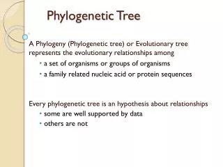
Phylogeny • A systematic and objective way to construct these trees is by comparing DNA/protein sequences • In this lecture, we study trees that relate objects that are sufficiently different • Different species • Different strains/populations of a species • Our goal is to reconstruct the actual evolutionary relationships based on observable sequences CSCI3220 Algorithms for Bioinformatics | Kevin Yip-cse-cuhk | Fall 2014
Assumptions • Basic assumptions behind phylogenetic trees: • The current sequences share a common ancestor • All were mutated from the common ancestor • Mutations are rare. Therefore if the DNA of A and B are more similar than both A and C as well as B and C, likely C was separated from A and B before their separation Common ancestor of A, B and C Common ancestor of A and B Time A B C CSCI3220 Algorithms for Bioinformatics | Kevin Yip-cse-cuhk | Fall 2014
Terminology • A tree is an acyclic graph with nodes connected by edges • A phylogenetic tree is a binary tree with sequences (nodes) connected by branches (edges) • Leaf nodes are the observed sequences • Internal nodes are the unobserved ancestral sequences • Branch lengths may represent evolutionary distances Branch length Root A leaf node An internal node A branch Image credit: Hershberg et al., Genome Biology 8:R164 (2007) , http://www.jdrf.ca/ CSCI3220 Algorithms for Bioinformatics | Kevin Yip-cse-cuhk | Fall 2014
Rooted and unrooted trees • Sometimes it is not very clear where the common ancestor should be put • We can have a tree without root – an unrooted tree Image credit: Lowery et al., Oncogene 24(2):248-259, (2005) CSCI3220 Algorithms for Bioinformatics | Kevin Yip-cse-cuhk | Fall 2014
Phylogenetic tree reconstruction • General problem: • Given a set of DNA/protein sequences • Find a phylogenetic tree such that it likely corresponds to the actual historical evolutionary events, involving: • Order of separation events (how the nodes are connected) • Ancestral sequences (what sequences the internal nodes have) • Branch lengths (how much time it has been since the separation) There are various ways to evaluate how likely a tree is correct. We will study them in this lecture • “Re”-construction: The tree was defined by history. We only try to reconstruct it from the observed sequences CSCI3220 Algorithms for Bioinformatics | Kevin Yip-cse-cuhk | Fall 2014
What sequence to use? • If we are studying a gene • DNA/protein sequence of the gene • If we want to know the relationship between different species • Whole genome (may not be feasible) • Some genes that are essential and single-copied • Ribosomal RNA CSCI3220 Algorithms for Bioinformatics | Kevin Yip-cse-cuhk | Fall 2014
Complexity of problem • Finding the “best” tree is a hard problem • How many tree topologies (i.e., ignore branch lengths and left-right order) are there for a set of k sequences? • For rooted trees: • k=2: 1 possible tree topology • k=3: 3 possible branches to add #3 • k=4: 5 possible branches to add #4, and so on • Therefore number of tree topologies is1 3 5 ... (2k-3) • Exponential 1 2 1 2 3 1 3 2 1 3 2 CSCI3220 Algorithms for Bioinformatics | Kevin Yip-cse-cuhk | Fall 2014
Complexity of problem • Similarly, for unrooted trees, • k=2: 1 possible tree topology • k=3: 1 possible branch to add #3 • k=4: 3 possible branches to add #4 • k=5: 5 possible branches to add #5 • There number of tree topologies is1 3 5 ... (2k-5) 4 1 1 1 4 1 1 3 3 3 3 2 2 2 2 4 2 CSCI3220 Algorithms for Bioinformatics | Kevin Yip-cse-cuhk | Fall 2014
Solving the problem: Ideas • What do you do when you encounter a computationally hard problem? • Define an easier version of the problem • By making certain assumptions • Design smart algorithms/data structures to avoid redundant calculations • Use heuristics to solve it, not necessarily getting the optical solution CSCI3220 Algorithms for Bioinformatics | Kevin Yip-cse-cuhk | Fall 2014
Phylogenetic tree reconstruction methods • Two main types of methods: • Sequence-based: need the sequences • Parsimony methods (easier problems, smart algorithms) • Probabilistic methods (easier problems, smart algorithms) • Maximum likelihood • Bayesian • ... • Distance-based: only depends on the distances • UPGMA (heuristics) • Neighbor joining (heuristics) • ... • We will study some of these algorithms CSCI3220 Algorithms for Bioinformatics | Kevin Yip-cse-cuhk | Fall 2014
The Newick format • Use brackets and comma to group two sub-trees • Use colon to indicate distance to parent • End with a semicolon Graphical representation: Newick: 1.00 ((((Homo:0.21,Pongo:0.21):0.28,Macaca:0.49):0.13,Ateles:0.62):0.38,Galago:1.00); 0.62 0.49 0.38 0.21 0.13 0.28 0.21 Image credit: http://www.zoology.ubc.ca/~schluter/zoo502stats/Rtips.phylogeny.html CSCI3220 Algorithms for Bioinformatics | Kevin Yip-cse-cuhk | Fall 2013
Part 2a Sequence-based Methods: Maximum Parsimony
Maximum parsimony • Assumption: A tree is likely to be true if it involves few mutations • Rationale: • Mutations are rare • “Occam’s razor”: The simplest explanation is likely the correct one • “Large parsimony” problem: • Given a set of sequences • Find a rooted tree topology of the sequences and the ancestral sequences of the tree • Such that the total number of mutations along the branches is minimized • NP hard: Currently no polynomial time algorithm is known • “Small parsimony” problem: • Given a set of sequences and a rooted tree topology of the sequences • Find the ancestral sequences • Such that the total number of mutations along the branches is minimized CSCI3220 Algorithms for Bioinformatics | Kevin Yip-cse-cuhk | Fall 2014
Small parsimony example • We will consider one single site • By assuming that sites are independent, we only need an algorithm for one site • Will show an example with more sites later • In the upper tree on the right, the number of mutations is 4 • Is it the minimum (i.e., most parsimonious solution)? • For this tree topology, the minimum number of mutations is 3. There are three sets of ancestral states that result in this number of mutations, shown in the three trees below G GC G GA C G CA GT A C G T A A A A A A A AG AT A G A T A A AC AC AC AT GT TG AG A C G T A A C G T A A C G T A CSCI3220 Algorithms for Bioinformatics | Kevin Yip-cse-cuhk | Fall 2014
Small parsimony problem • How to assign ancestral states so that the total number of mutations is minimized? • Ideas: For a given node, • If both children have the same state, probably good to adopt the state • If the two children have different states, probably good to adopt one of them • Delay the decision of the exact choice until the parent has also expressed a preference CSCI3220 Algorithms for Bioinformatics | Kevin Yip-cse-cuhk | Fall 2014
The algorithm: simple version • Fitch’s algorithm: If you only need some solutions • For each internal node i with parent p and children l and r, we will determine its preference set Si and its final character Ci that would minimize the total number of mutations • Steps: • For each leaf node i, set Si to the character of the sequence • Upward phase: For each internal node i,if (Sl Sr)={}// l and r do not agree: take both sets Si := Sl Sr else// l and r agree on something: take it Si := Sl Sr • Downward phase: First pick any Croot from Sroot. Then for each other internal node i, if Cp Si// p agrees with i on something: take it Ci := Cpelse // p disagrees with i: use i’s own preferences Ci := choose one from Si p i r l CSCI3220 Algorithms for Bioinformatics | Kevin Yip-cse-cuhk | Fall 2014
An example A A,G,T Upward phase A,C G,T A C G T A A C G T A Downward phase (2 choices) A A A A,G,T A A OR A,C G,T A T A G A C G T A A C G T A CSCI3220 Algorithms for Bioinformatics | Kevin Yip-cse-cuhk | Fall 2014
Why does it work? • Proof by induction • When there are only two leaves, there are two cases: • They have the same character • Actual minimum number of mutations: 0 • The algorithm gives the same number • They have different characters • Actual minimum number of mutations: 1 • The algorithm gives the same number A A A A A A A C A C C A C CSCI3220 Algorithms for Bioinformatics | Kevin Yip-cse-cuhk | Fall 2014
Why does it work? • Assume the algorithm is able to minimize the number of mutations for k or fewer leaves • Now for a tree with k+1 leaves, • It consists of a root connected to two sub-trees with roots l and r, both with k or fewer leaves • Two cases: • If Sl Sr {}, the algorithm gives a solution with ml + mr mutations, which is optimal due to the induction hypothesis • If Sl Sr = {}, the algorithm gives a solution with ml + mr + 1 mutations, which is also optimal since one extra mutation must be introduced between the root and one of its children root r l ... ... ... ... Minimum number of mutations: ml Minimum number of mutations: mr CSCI3220 Algorithms for Bioinformatics | Kevin Yip-cse-cuhk | Fall 2014
The algorithm: extended version • If you need all solutions • Steps: • For each leaf node i, set Si to the character of the sequence • Upward phase (same as before): For each internal node i,if (Sl Sr)={}// l and r do not agree: take both sets Si := Sl Sr else// l and r agree on something: take it Si := Sl Sr • Downward phase: First pick Croot from Sroot. Then for each other internal node i(different strategy -- majority vote): we will choose Ci from the characters that exist in the largest number of sets among {Cp}, Sl and Sr • We can prove that this algorithm gives all optimal solutions • A special case of Sankoff’s dynamic programming algorithm p i r l CSCI3220 Algorithms for Bioinformatics | Kevin Yip-cse-cuhk | Fall 2014
Revisiting the same example A A,G,T Upward phase A,C G,T A C G T A A C G T A Downward phase (3 choices) A A A A A A OR OR A G A A T A A C G T A A A C C G G T T A A CSCI3220 Algorithms for Bioinformatics | Kevin Yip-cse-cuhk | Fall 2014
A more complex example A,C,G G A,C,G A,C,G A,C,G A,C,G A,C,G A,C,G Upward phase A,G G G G G G G A,C A A,G A,G A,G A,G A,G A,G A,C A,C A,C A,C A,C A,C A A A A A A A A A A A A A A C C C C C C C C A A A A A A A A A A A A A A A A G G G G G G G G G G G G G G G G Downward phase (6 choices) A A C A G G A G G A A A A C A G G G G G G G G G A A C A G A CSCI3220 Algorithms for Bioinformatics | Kevin Yip-cse-cuhk | Fall 2014
Multiple sites • In a real situation, we need to deal with sequences that contain more than one site • We simply apply the above algorithm to the different sites independently • As we assume that different sites mutate independently CSCI3220 Algorithms for Bioinformatics | Kevin Yip-cse-cuhk | Fall 2014
Example [G][C,T] • Minimum: 1 substitution for position 1, 1 substitution for position 2 • Maximum parsimony: 2 trees that can achieve such minimum [G][C,T] [G][C,T] Upward phase [A,G][C] [A,G][C] [A,G][C] AC GC GT AC AC AC GC GC GC GT GT GT Downward phase GC GT OR GC GC CSCI3220 Algorithms for Bioinformatics | Kevin Yip-cse-cuhk | Fall 2014
From small parsimony to large parsimony • Some heuristic methods try different tree topologies. For each one, solve the small parsimony problem. Then compare and find the best. • A standard “searching problem” in AI • Need ways to: • Determine the first trees • Determine the next trees based on the current tree • Avoid trapping in a local optimum • There are many methods proposed for these tasks CSCI3220 Algorithms for Bioinformatics | Kevin Yip-cse-cuhk | Fall 2014
Part 2b Sequence-based Methods: Maximum Likelihood
Evolutionary distance • Suppose we have an alignment of two sequences. At a site, one sequence has an A and one has a C. • Assume that the sequences have a common ancestor • What did the common ancestor have at that site? • We don’t know. • Let’s say A. How many mutations have happened? • Could be one (AC) • Could be more (AGC, ATC, ACA, etc.) • We want a way to define the “evolutionary distance” between two observed sequences • According to the number of mutations happened or the time since their divergence • We need to first define a mutation model TTAGG TTCGG TT?GG TTAGG TTAGG TTAGG TTCGG TTCGG TTAGG TTAGG TTGGG TTCGG CSCI3220 Algorithms for Bioinformatics | Kevin Yip-cse-cuhk | Fall 2014
Technical assumptions • These assumptions are usually not true, but they will greatly simplify the problem: • Sites are independent • Mutation rates are the same for different sites and at different time in the history • Given current state, future states do not depend on past states • Markov property! • More complex models that require fewer strong assumptions exist. We only study the simple models here CSCI3220 Algorithms for Bioinformatics | Kevin Yip-cse-cuhk | Fall 2014
The Jukes-Cantor model • Proposed by Jukes and Cantor in 1969 • Equal rate of substitution, , to the other three bases in one unit of time • Assume there is at most one mutation within one unit of time – We can always make the unit smaller to ensure this 1-3 1-3 A G C T 1-3 1-3 CSCI3220 Algorithms for Bioinformatics | Kevin Yip-cse-cuhk | Fall 2014
Illustration of the Jukes-Cantor model • Suppose at time 0, site 1 of a sequence was A • At time 1: • There is a probability of 1-3 that the site was A • There is a probability of that the site was C • There is a probability of that the site was G • There is a probability of that the site was T • At time 2, what is the probability that the site is A? • Two possibilities: • At time 1, the site was A, and there was no mutation from time 1 to time 2 [probability: (1-3)2] • At time 1, the site was C, G or T, and there was a mutation to A from time 1 to time 2 [probability: 32] • Therefore, the total probability that the site is A at time 2 is (1-3)2 + 32 CSCI3220 Algorithms for Bioinformatics | Kevin Yip-cse-cuhk | Fall 2014
Recursive formulas • Denote PXY(t) as the probability that for a base that was X at time 0, it is Y at time t, for any X and Y • Here “site”, “base”, “nucleotide” all mean the same thing • PAA(1) = 1 - 3 • PAA(2) = (1 - 3)2 + 32 • In general,PAA(t+1) = (1 - 3)PAA(t) + [1 - PAA(t)] • Similarly: • PXX(t+1) = (1 - 3)PXX(t) + [1 - PXX(t)] for any X • PXY(t+1) = [1 - PXX(t+1)] / 3 for any X and Y CSCI3220 Algorithms for Bioinformatics | Kevin Yip-cse-cuhk | Fall 2014
Solving the equation • (Suggested by your classmate Cao Jianquan when he took BMEG3102) • PAA(t) = (1 - 3)PAA(t-1) + [1 - PAA(t-1)] = (1 - 4)PAA(t-1) + PAA(t) - 1/4 = (1 - 4)PAA(t-1) + - 1/4 = (1 - 4)PAA(t-1) - 1/4 (1 - 4) = (1 - 4)(PAA(t-1) - 1/4) = (1 - 4)2(PAA(t-2) - 1/4) = ... = (1 - 4)t-1(PAA(1) - 1/4) = (1 - 4)t-1(1 - 3 - 1/4) = (1 - 4)t-1(3/4 - 3) = 3/4 (1 - 4)t PAA(t) = 3/4 (1 - 4)t + 1/4 CSCI3220 Algorithms for Bioinformatics | Kevin Yip-cse-cuhk | Fall 2014
Maximum likelihood • Likelihood: Probability of producing the observed data by a model given the model parameters, Pr(X|) • X: Observed data • The input sequences, assumed aligned • Again, we consider one single site here. The likelihood for the whole sequences is the product of the likelihood of individual sites since they are assumed independent • : Model parameters (see next page) • Maximum likelihood: Find value of such that Pr(X|) is maximized CSCI3220 Algorithms for Bioinformatics | Kevin Yip-cse-cuhk | Fall 2014
Model parameters • There are different possibilities • In all cases, X is the input sequences • Big likelihood problem • : tree topology, mutation rates and divergence times • Very difficult • Small likelihood problem • Tree topology is given • : mutation rates and divergence times • There are effective heuristic solutions that usually (but not always) produce optimal results CSCI3220 Algorithms for Bioinformatics | Kevin Yip-cse-cuhk | Fall 2014
Computing likelihood • Suppose we are given the followings, as shown in the figure: • Tree topology • Observed data, X = {a:G, b:G, c:T, d:G} • Ancestral sequences • Parameters, = {<mutation rates>, tae, tbe, tcf, tdf, teg, tfg} • Likelihood =Pr(g:G)Pr(e:G|g:G, teg) Pr(f:G|g:G, tfg)Pr(a:G|e:G, tae) Pr(b:G|e:G, tbe)Pr(c:T|f:G, tcf) Pr(d:G|f:G, tdf) • We have learned how to compute these conditional probabilities for the Jukes-Cantor model • Noticed the Markov property used here? g:G teg tfg e:G f:G tae tbe tcf tdf a:G b:G c:T d:G Node labels Observed sequences Ancestral sequences : Divergence times CSCI3220 Algorithms for Bioinformatics | Kevin Yip-cse-cuhk | Fall 2014
Computing likelihood • In the small likelihood problem, we are only given the tree topology, but not the ancestral sequences – Then how to compute likelihood? • Need to try them all: Likelihood =Pr(g:A)Pr(e:A|g:A, teg) Pr(f:A|g:A, tfg)Pr(a:G|e:A, tae) Pr(b:G|e:A, tbe)Pr(c:T|f:A, tcf) Pr(d:G|f:A, tdf)+Pr(g:C)Pr(e:A|g:C, teg) Pr(f:A|g:C, tfg)Pr(a:G|e:A, tae) Pr(b:G|e:A, tbe)Pr(c:T|f:A, tcf) Pr(d:G|f:A, tdf)+...+Pr(g:T)Pr(e:T|g:T, teg) Pr(f:T|g:T, tfg)Pr(a:G|e:T, tae) Pr(b:G|e:T, tbe)Pr(c:T|f:T, tcf) Pr(d:G|f:T, tdf) g:? teg tfg e:? f:? tae tbe tcf tdf a:G b:G c:T d:G Possible ancestral states: CSCI3220 Algorithms for Bioinformatics | Kevin Yip-cse-cuhk | Fall 2014
Computational efficiency • How much computation is needed? • For our example: • 3 internal node 43 = 64 possible sets of ancestral states • For each set of ancestral states, we need to multiply 7 terms (because there are 7 nodes in the tree) • In general: • If there are n input sequences, there are n-1 internal nodes 4n-1 possible sets of ancestral states • For each set of ancestral states, we need to multiply n+n-1 = 2n-1 terms • Impractical to perform this exponential number of operations • You must know how to deal with this situation by now – dynamic programming! CSCI3220 Algorithms for Bioinformatics | Kevin Yip-cse-cuhk | Fall 2014
Computing likelihood efficiently • An important observation: once the root of a sub-tree is determined, the likelihood of this sub-tree does not depend on other nodes in the whole tree • Once node e is decided to take character A, the likelihood of the sub-tree involving nodes a, b and e is alwaysPr(e:A)Pr(a:G|e:A, tae)Pr(b:G|e:A, tbe) g:? teg tfg e:A f:? tae tbe tcf tdf a:G b:G c:T d:G CSCI3220 Algorithms for Bioinformatics | Kevin Yip-cse-cuhk | Fall 2014
Computing likelihood efficiently • Define table V, where entry V(i,x) is the likelihood of the sub-tree rooted at i when the parent of i takes character x • Likelihood =Pr(g:A) V(e,A) V(f,A) +Pr(g:C) V(e,C) V(f,C) +Pr(g:G) V(e,G) V(f,G) +Pr(g:T) V(e,T) V(f,T) • V(e, A) =Pr(e:A|g:A,teg) V(a,A) V(b,A) +Pr(e:C|g:A,teg) V(a,C) V(b,C) +Pr(e:G|g:A,teg) V(a,G) V(b,G) +Pr(e:T|g:A,teg) V(a,T) V(b,T) • V(a,A) = Pr(a:G|e:A, tae) • V(a,C) = Pr(a:G|e:C, tae) • ... • Table V contains O(n) entries. Computing the value for each entry requires a constant number of operations Linear time overall g:? teg tfg e:? f:? tae tbe tcf tdf a:G b:G c:T d:G CSCI3220 Algorithms for Bioinformatics | Kevin Yip-cse-cuhk | Fall 2014
Example e:? tde tce • Let’s assume: • All four bases are equally likely at the root • The Jukes-Cantor mutation model is correct • Mutation rate per unit time, =0.1 • Each branch in the tree represents one unit of time • V(i,x) is the likelihood of the sub-tree rooted at i when the parent of i takes character x • Overall likelihood: 0.25(0.058)(0.1) + 0.25(0.058)(0.1) + 0.25(0.022)(0.7) + 0.25(0.022)(0.1) = 0.0073 d:? tad tbd a:A b:C c:G CSCI3220 Algorithms for Bioinformatics | Kevin Yip-cse-cuhk | Fall 2014
Solving the small likelihood problem • Then how to find the optimal parameter values? • Start with a random estimate of • Apply a “hill climbing” algorithm • Change the value of a parameter so that the likelihood is increased • Repeat it for each parameter in turn, for multiple iterations • Will reach maximum if there is a single “peak” – This is true in many real situations, though theoretically cases can be constructed in which this it not true (For simplicity, assume ={, tab} here) New estimate Current estimate Likelihood tab a Image source: http://www.absoluteastronomy.com/topics/Hill_climbing CSCI3220 Algorithms for Bioinformatics | Kevin Yip-cse-cuhk | Fall 2014
Part 3a Distance-based Methods: UPGMA
Motivation • In the previous sequence-based algorithms, the exact sequences are used when reconstructing the phylogenetic trees • In a sequence-based method, only the pairwise distances between the sequences are considered • Good if the sequences are long, and we care only about the tree structure but not the ancestral sequences • The distances can be computed by methods based on sequence alignment • Once the pairwise distances have been computed, the original sequences will not be used CSCI3220 Algorithms for Bioinformatics | Kevin Yip-cse-cuhk | Fall 2014
UPGMA • Unweighted Pair Group Method with Arithmetic Mean • Algorithm: • Compute the distance between each pair of sequences • Treat each sequence as a cluster by itself • Merge the two closest clusters. The distance between two clusters is the average distance between all their sequences (except that d(Ci, Ci)=0): • Repeat 2 and 3 until only one cluster remains CSCI3220 Algorithms for Bioinformatics | Kevin Yip-cse-cuhk | Fall 2014