Download
1 / 43
500 likes | 1.26k Views
INITIAL LAYOUT CONSTRUCTION. Preliminaries From-To Chart / Flow-Between Chart REL Chart Layout Scores Traditional Layout Construction Manual CORELAP Algorithm Graph-Based Layout Construction REL Graph, REL Diagram, Planar Graph Layout Graph, Block Layout

E N D
INITIAL LAYOUT CONSTRUCTION • Preliminaries • From-To Chart / Flow-Between Chart • REL Chart • Layout Scores • Traditional Layout Construction • Manual CORELAP Algorithm • Graph-Based Layout Construction • REL Graph, REL Diagram, Planar Graph • Layout Graph, Block Layout • Heuristic Algorithm to Construct a REL Graph • General Procedure
Given M activities, a From-To Chart represents M(M-1) asymmetric quantitative relationships. Example: where fij = material flow from activity i to activity j. A Flow-Between Chart represents M(M-1)/2 symmetric quantitative relationships, i.e., gij = fij + fji, for all i > j, where gij = material flow between activities i and j. f f f f f f 12 13 23 32 21 31 From-To and Flow-Between Charts
A Relationship (REL) Chart represents M(M-1)/2 symmetric qualitative relationships, i.e., where rij{A, E, I, O, U}: Closeness Value (CV) between activities i and j; rij is an ordinal value. A number of factors other than material handling flow (cost) might be of primary concern in layout design. rij values when comparing pairs of activities: A = absolutely necessary 5 % E = especially important 10 % I = important 15 % O = ordinary closeness 20 % U = unimportant 50 % X = undesirable 5 % V(rij) = arbitrary cardinal value assigned to rij, e.g., V(U) = 1, etc. r 12 r 13 r 23 Relationship (REL) Chart
2 1 4 3 5 Adjacency • Two activities are (fully) adjacent in a layout if they share a common border of positive lenght, i.e., not just a point. • Two activities are partially adjacent in a layout if they only share one or a finite number of points, i.e., zero length. • Let aij [0, 1]: adjacency coefficient between activities i and j. • Example: (Fully) adjacent: a12 = a13 = a24 = a34 = a45 = 1, Partially adjacent: a14 = a23 = a25 = , and Non-adjacent: a15 = a25 = 0.
Layout Scores Two ways of computing layout scores: • Layout score based on distance: where dij = distance between activities i and j. • Layout score based on adjacency: where aij [0, 1]: adjacency coefficient between activities i and j.
Legend A Rating E Rating I Rating O Rating U Rating X Rating Traditional Layout Configuration • An Activity Relationship Diagram is developed from information in the activity relation chart. Essentially the relationship diagram is a block diagram of the various areas to be placed into the layout. • The departments are shown linked together by a number of lines. The total number of lines joining departments reflects the strength of the relationship between the departments. E.g., four joining lines indicate a need to have two departments located close together, whereas one line indicates a low priority on placing the departments adjacent to each other. • The next step is to combine the relationship diagram with departmental space requirements to form a Space Relationship Diagram. Here, the blocks are scaled to reflect space needs while still maintaining the same relative placement in the layout. • A Block Plan represents the final layout based on activity relationship information. If the layout is for an existing facility, the block plan may have to be modified to fit the building. In the case of a new facility, the shape of the building will confirm to layout requirements.
REL chart: 1. Offices 2. Foreman 3. Conference Room 4. Parcel Post 5. Parts Shipment 6. Repair and Service Parts 7. Service Areas 8. Receiving 9. Testing 10. General Storage O 4 I 5 U U U E 3 U U E 3 E 5 O 4 U O 4 U U E3 A 1 O 3 I 2 U U U I 4 U U I 2 U U U U Code Reason 1 Flow of material 2 Ease of supervision 3 Common personnel 4 Contact Necessary 5 Conveniences U I 2 U U A 1 U O 2 U I 1 U I 2 U U I 2 U Rating Definition A Absolutely Necessary E Especially Important I Important O Ordinary Closeness OK U Unimportant X Undesirable Example
8 7 5 10 9 6 4 2 3 1 Example (Cont.) Activity Relationship Diagram
7 (575) 5 (500) 8 (200) 9 (500) 6 (75) 10 (1750) 3 (125) 4 (350) 2 (125) 1 (1000) Space Relationship Diagram Example (Cont.)
Manual CORELAP Algorithm • CORELAP is a construction algorithm to create an activity relationship (REL) diagram or block layout from a REL chart. • Each department (activity) is represented by a unit square. • Numerical values are assigned to CV’s: V(A) = 10,000, V(O) = 10, V(E) = 1,000, V(U) = 1, V(I) = 100, V(X) = -10,000. • For each department, the Total Closeness Rating (TCR) is the sum of the absolute values of the relationships with other departments.
Procedure to Select Departments 1. The first department placed in the layout is the one with the greatest TCR value. I|f a tie exists, choose the one with more A’s. 2. If a department has an X relationship with he first one, it is placed last in the layout. If a tie exists, choose the one with the smallest TCR value. 3. The second department is the one with an A relationship with the first one. If a tie exists, choose the one with the greatest TCR value. 4. If a department has an X relationship with he second one, it is placed next-to-the-last or last in the layout. If a tie exists, choose the one with the smallest TCR value. 5. The third department is the one with an A relationship with one of the placed departments. If a tie exists, choose the one with the greatest TCR value. 6. The procedure continues until all departments have been placed.
8 6 7 0 1 5 2 3 4 Procedure to Place Departments • Consider the figure on the right. Assume that a department is placed in the middle (position 0). Then, if another department is placed in position 1, 3, 5 or 7, it is “fully adjacent” with the first one. It is placed in position 2, 4, 6 or 8, it is “partially adjacent”. • For each position, Weighted Placement (WP) is the sum of the numerical values for all pairs of adjacent departments. • The placement of departments is based on the following steps: 1. The first department selected is placed in the middle. 2. The placement of a department is determined by evaluating all possible locations around the current layout in counterclockwise order beginning at the “western edge”. 3. The new department is located based on the greatest WP value.
1. Receiving 2. Shipping 3. Raw Materials Storage 4. Finished Goods Storage 5. Manufacturing 6. Work-In-Process Storage 7. Assembly 8. Offices 9. Maintenance 1. Receiving 2. Shipping 3. Raw Materials Storage 4. Finished Goods Storage 5. Manufacturing 6. Work-In-Process Storage 7. Assembly 8. Offices 9. Maintenance A A E E A O E U U A U O E U A U O E O U A U A E A A E A U O A O X O A X Example CV values: V(A) = 125 V(E) = 25 V(I) = 5 V(O) = 1 V(U) = 0 V(X) = -125 Partial adjacency: = 0.5
62.5 187.5 187.5 62.5 125 62.5 62.5 5 7 7 125 125 125 125 62.5 125 62.5 62.5 187.5 187.5 62.5 62.5 125.5 63.5 1 0 62.5 125 62.5 0 5 7 3 5 7 125 0 0 187.5 9 9 62.5 126.5 1.5 0 0 187.5 187.5 0.5 1 0.5 62.5 125 62.5 Example (cont.)
12.5 37.5 100 137.5 62.5 3 5 7 37.5 125 1 9 37.5 137.5 62.5 12.5 25 12.5 0 0 62.5 125 188 62.5 3 5 7 0.5 1 125 2 1 9 4 1 63.5 0.5 1 1 1.5 1.5 0.5 Example (cont.) 12.5 25 12.5 0 0 3 5 7 87.5 62.5 1 9 4 137.5 125 62.5 125 125 125 62.5
0.5 0.5 1 0.5 6 6 12.5 25.5 -60.5 -61.5 3 5 7 8 3 5 7 12.5 112.5 -112 2 1 9 4 2 1 9 4 25 -37.5 12.5 87.5 75 -62.5 -37.5 12.5 Example (cont.)
Nonplanar Planar Planar Graph • Assumption: • A Planar Graph is a graph that can be drawn in two dimensions with no arc crossing. • A graph is nonplanar if it contains either one of the two Kuratowski graphs:
1 2 2 1 3 4 5 3 4 5 6 Relationship (REL) Graph • Given a (block) layout with M activities, a corresponding planar undirected graph, called the Relationship (REL) Graph, can always be constructed. (Exterior) Block Layout REL Graph • A REL graph has M+1 nodes (one node for each activity and a node for the exterior of the layout. The exterior can be considered as an additional activity. The arcs correspond to the pairs of activities that are adjacent. • A REL graph corresponding to a layout is planar because the arcs connecting two adjacent activities can always be drawn passing through their common border of positive length.
Relationship (REL) Diagram • A Relationship (REL) Diagram is also an undirected graph, generated from the REL chart, but it is in general nonplanar. • A REL diagram, including the U closeness values, has M(M-1)/2 arcs. Since a planar graph can have at most 3M-6 arcs, a REL diagram will be nonplanar if M(M-1)/2 > 3M-6. M(M-1)/2 > 3M-6 M 5. • A REL graph is a subgraph of the REL diagram. • For M 5, at most 3M-6 out of M(M-1)/2 relationships can be satisfied through adjacency in a REL graph. An upper bound on LSa, LSaUB, is the sum of the 3M-6 longest V(rij)’s.
Maximally Planar Graph (MPG) • A planar graph with exactly 3M-6 arcs is called Maximally Planar Graph (MPG). Not MPG since has only 5 arcs (5 < 6 = 3M-6) MPG since has 6 arcs • The interior faces of a graph are the bounded regions formed by its arcs, and its exterior face is the unbounded region formed by its outside arcs. The tetrahedron has three interior faces (IF1, IF2 and IF3) and an exterior face (EF) EF IF1 IF2 IF3
Maximally Planar Graph (MPG) • The interior faces and the exterior face of an MPG are triangular, i.e., the faces are formed by three arcs. Not triangular Not an MPG • The REL graph of a given a (block) layout may not be an MPG. Not an MPG REL Graph Layout
Maximally Planar Weighted Graph (MPWG) • An MPG whose sum of arc weights is as large as any other possible MPG is called a Maximally Planar Weighted Graph (MPWG). • Using the V(rij)’s as arc weights, a REL graph that is a MPWG has the maximum possible LSa, close to LSaUB. • Since it is difficult to find an MPWG, a Heuristic (non-optimal) procedure will be used to construct a REL graph that is an MPG, but may not be an MPWG (although its LSa will be close to LSaUB). • The Layout Graph is the dual of the REL graph. • Given a graph G, its dual graph GD has a node for each face of G and two nodes in GD are connected with an arc if the two corresponding faces in G share an arc.
GD G Layout Graph • Example. • The number of nodes in G (primal graph) is the same than the number of faces in GD (dual graph), and vice versa. In addition, (GD)D = G. • Primal Graph is Planar Dual Graph is planar.
1 2 3 4 5 Layout Graph (Cont.) • Given a layout, the corresponding layout graph can always be constructed by placing the nodes at the corners of the layout where three or more activities meet (including the exterior of the layout as an activity). The arcs in the graph are the remaining portions of the layout walls. E.g., a b Only activity 3 and exterior meet here e c g Activities 3, 5, and exterior meet here d f h (Exterior) Layout Graph Layout • Given a REL graph (RG), its corresponding layout graph (LG) is LG = RGD. E.g., 6 RGD 2 3 1 5 4 LGD RG LG
Layout Graph (Cont.) • If LG is given, then RG = LGD, but for layout construction, the layout is not known initially, so LG cannot be constructed without RG. • If a planar REL graph (primal graph) exist, the corresponding layout graph (dual graph) is also planar. Therefore, it is possible theorectically to construct a block layout that will satisfy all the adjacency requirements. In practice, this is not straightforward because the space requirements of the activities are difficult to handle.
Example REL graph (Primal graph): Space Requirements: Dept. Area A 300 B 200 C 100 D 200 E 100 F (exterior) A B E F C D
A B 1 E F 2 3 4 5 7 6 8 C D Example (Cont.) Layout graph (Dual graph):
Example (Cont.) Square Block Layout: (areas are not considered) Block Layout: 8 4 A B E A 8 1 6 1 5 F C B 8 2 3 F C D 7 2 3 4 D E 5 7 • A corner point is a point where at least three departments meet, including the exterior department. • Note that each corner point in the block layout corresponds to a node in the layout graph. In the first block layout, each corner point is defined by “exactly” three departments. In this case, there is a one-to-one correspondence between corner points and nodes in the layout graph. In the square block layout, there are two corner points defined by four departments, i.e., (A, B, C, D) and (B, D, E, F). Each of these two corner points corresponds to two nodes in the layout graph.
Heuristic Procedure to Construct a Relationship Graph 1. Rank activities in non-increasing order of TCRk, k = 1, …,M, where TCRk = (Note that the negative values of V(rik) and V(rkj) are not included in TCRk). 2. Form a tetrahedron using activities 1 to 4 (i.e., the activities with the four largest TCRk‘s). 3. For k = 5, …, M, insert activity k into the face with the maximum sum of weights (V(rij)) of k with the three nodes defining the face (where “insert” refers to connecting the inserted node to the three nodes forming the face with arcs). 4. Insert (M+1)th node into the exterior face of the REL graph.
A B C D E F I O X I O U A U U E E U E E O Example REL chart: CV values: V(A) = 81 V(E) = 27 V(I) = 9 V(O) = 3 V(U) = 1 V(X) = -243
A O A I = rAD V(rAD) = 9 C E U E F D Example (Cont.) Step 2:
EF Face LSa EF 9 + 1 + 27 = 37 * IF1 9 + 27 - 243 = -207 IF2 9 - 243 + 1 = -233 IF3 27 - 243 + 1 = -215 Insert B in EF A I IF3 IF2 IF1 I I X C X E E X U E U F D U Example (Cont.) Step 3: Insert B.
Example (Cont.) Face LSa EF 5 IF1 7 IF2 33 * IF3 31 IF4 31 IF5 5 Insert E in IF2 Step 3 (Cont.): Insert E. A B EF IF1 IF3 IF2 C IF4 F D IF5
A B EX E C F D Example (Cont.) Step 4: Call exterior activity EX. Since arcs (AB), (BD), and (DA) are the outside arcs, EX connects to nodes A, B, and D.
Example (Cont.) • LSaUB is the sum of the 3M - 6 ( 3 6 - 6 = 12), largest V(rij)’s. In the last example, LSaUB = V(rAF) + V(rBF) + V(rCE) + V(rCF) + V(rDF) + V(rAB) + V(rAD) + V(rAC) + V(rAE) + V(rEF) + V(rBD) + V(rBE) = 81 + 27 + 27 + 27 + 27 + 9 + 9 + 3 + 3 + 3 + 1 + 1 = 218. • For the final REL graph, LSa = 218. • LSaUB = LSa The final REL graph is an MPWG It is optimal. • LSaUB > LSa The final REL graph may not be an MPWG It may not be optimal. • Using the Heuristic procedure, the generated REL graph will always be an MPG since each face is triangular.
REL Chart REL Graph Layout Graph Initial Layout Space Requirements General Procedure for Graph Based Layout Construction 1. Given the REL chart, use the Heuristic procedure to construct the REL graph. 2. Construct the layout graph by taking the dual of the REL graph, letting the facility exterior node of the REL graph be in the exterior face of the layout graph. 3. Convert (by hand) the layout graph into an initial layout taking into consideration the space requirement of each activity.
A B EX E C F D REL Graph Example Step 1: (from before)
A B EX E C F D Layout Graph Example (Cont.) Step 2: take the dual of RG
A E C B D F Initial Layout Example (Cont.) Step 3: • Initial layout is drawn as a square, but could be any other shape. • Only A and B are nonrectangular.
Comments 1. If an activity is desired to be adjacent to the exterior of a facility (e.g., a shipping/receiving department), then the exterior could be included in the REL chart and treated as a normal activity, making sure that, in step 1 of the general procedure, its node is one of the nodes forming the exterior face of the REL graph. 2. The area of each interior face of the layout graph constructed in step 2 does not correspond to the space requirements of its activity. 3. In step 3, the overall shape of the initial layout should be usually be rectangular if it corresponds to an entire building because rectangular buildings are usually cheaper to build; even if the initial layout corresponds to just a department, a rectangular shape would still be preferred, if possible. 4. In step 3, the shape of each activity in the initial layout should be rectangular if possible, or at most L- or T-shaped (e.g., activities A and B), because rectangular shapes require less wall space to enclose and provide more layout possibilities in interiors as compared to other shapes.
Comments (Cont.) 5. All shapes should be orthogonal, i.e., all corners are either 90 or 270 (e.g., a triangle is not an orthogonal shape since its corners could all be 60). 6. In step 1, if the LSa of the REL graph is less than LSaUB, then the REL graph may not be optimal. The following three steps may improve the REC graph for the purpose of increasing LSa: a) Edge Replacement: replace an arc in the REL graph with a new arc not previously in the graph, without losing planarity, if it increases LSa. b) Vertex Relocation: move a node in the REL graph connected to three arcs to another triangular face if it increases LSa. c) Use a different activity to replace one of the four activities of the tetrahedron formed in step 2 of the Heuristic procedure to construct a new REL graph.