Download
1 / 19
190 likes | 196 Views
Intro to Deterministic Analysis. Deterministic network calculus: Theory for obtain worst-case (=deterministic) network performance Developed in the 1990s ( Rene Cruz ) Bounds of interest: Delay at a switch Backlog at a switch Traffic at output of switch. Components of a Packet Switch.

E N D
Intro to Deterministic Analysis left-continuous
Deterministic network calculus: • Theory for obtain worst-case (=deterministic) network performance • Developed in the 1990s (Rene Cruz) • Bounds of interest: • Delay at a switch • Backlog at a switch • Traffic at output of switch
Modeling a packet switch Model with input and output buffers
Modeling a packet switch Model with input and output buffers Simplified model (only output buffers)
Model of a switch Buffering takes place only at the output. (Neglect processing delay)
Store and Forward: Packet arrives to buffer only after all bytes of the packet have been received An arrival to the buffer appears instantaneous Multiple packets can arrive at the same time Scheduling Algorithms: FIFO Priority Round-Robin Earliest-Deadline-First Packet arrivals
Modeling Traffic Arrivals • We write arrivals as functions of time: A(t) : Arrivals until time t, measured in bits • There are a number of choices to be made: • Continuous time or Discrete time domain • Discrete sized or fluid flow traffic • Left-continuous or right-continuous
Continuous time vs. Discrete time Domain • Continous time: t is a non-negative real number • Discrete time: Time is divided in clock ticks t = 0,1,2, ….
Discrete-sized vs. Fluid flow • It is often simpler to view traffic as a fluid flow, that allows discrete sized bursts Traffic arrives in multiples of bits Traffic arrives like a fluid
Left-continuous vs. right-continuous • With instantaneous (discrete-sized) arrivals in a continuous time domain, the arrival function A is a step function • There is a choice to draw the step function: ECE 1545
Left-continuous vs. right-continuous right-continuous left-continuous • We will use a left-continuous arrival function A(t) considers arrivals in (0,t] A(t) considers arrivals in [0,t)(Note: A(0) = 0 !)
Arrivals of packets to a buffered link • Backlog at the buffered link
Link rate of output is C Packet length is up to L bits long Assumptions: Scheduler is work-conserving (always transmitting when there is a backlog) Infinite Buffers slope C Backlog Backlog ECE 1545
Definitions: ECE 1545
Dealing with instantaneous arrivals • If we have an instantaneous arrival, then the arrival function is a step function. • Need to decide which time the arrival takes place. • We assume that the arrival occurs at time t+ • This leads to a left-continuous arrival function. ECE 1545