Objectives to understand:

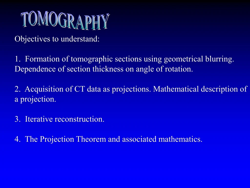
1. TOMOGRAPHY Objectives to understand: 1. Formation of tomographic sections using geometrical blurring. Dependence of section thickness on angle of rotation. 2. Acquisition of CT data as projections. Mathematical description of a projection. 3. Iterative reconstruction. 4. The Projection Theorem and associated mathematics.

2. Tomography objectives (continued): 5. Filtered Back Projection and associated mathematics. 6. CT exposure requirements. 7. Definition of CT image values. 8. Spiral CT and CT angiography.

3. Introduction In conventional radiographic projection imaging, the attenuation effects from material situated throughout the x-ray path are superimposed at the detector plane, as shown below. Detector Source •

4. This can lead to considerable ambiguity, for example when a low contrast object is superimposed on a dense or anatomically complex object. The object of tomography is to obtain images corresponding to the attenuation distribution within a planar section through the body. Another problem with conventional radiographic projection imaging is the presence of x-ray scatter, which makes it difficult to make quantitative assessment of attenuation values. The first of these problems was addressed by conventional film tomography sometimes called blurring tomography. Eventually, both were addressed by computed tomography (CT).

5. First let us consider the blurring approach which was introduced circa 1930 by Ziedses Des Plantes in Holland (in the same PhD thesis which introduced film subtraction angiography--try to beat that when you choose your thesis topic!)

6. A B A B A Conventional Blurring Tomography The basic geometry for blurring tomography is shown in below. Source motion A B • • Detector motion

7. A and B are objects at two different depths within the patient. By coordinating the motion of the detector and the source, objects such as A in the plane of rotation remain stationary on the detector. Objects such as B, which are outside the plane of rotation, are smeared out as the source and detector are rotated. The degree of blurring increases with the angle of rotation. Therefore the thickness of the in-focus plane decreases with increased rotation.

8. Several different types of blurring may be used. For example, linear, circular or hypocycloidal motions are used and result in different characteristic blurring artifacts. The choice of motion is made by considering which type of artifact is less likely to mimic the anatomy which may be under study.

9. Figure 3A below shows a frontal conventional radiograph of the head. In Figure 3B, blurring tomography has been used to select a plane through the maxillary sinuses. The arrows point to a mass in one of the maxillary sinuses. A B

10. Computed Tomography In computed tomography, x-rays pass in a direction approximately transverse to the longitudinal axis of the body and pass only through the slice of interest, thus overcoming the problem of overlapping information from adjacent slices. The goal is to obtain an image representing the two dimensional distribution of attenuation coefficients at each picture element in the image. Various mathematical schemes may be used to reconstruct the image from the projection information.

11. An advantage of the slice geometry, analogous to that of the line scanned x-ray systems discussed in the section on scatter, is that scatter is greatly reduced. Additionally, in CT, electronic detectors capable of quantitative recording of the transmitted information are used. These two factors were essential in providing the revolutionary contrast resolution made available by CT in the mid 1970’s.

12. Figure 4 illustrates the concept of projection data. At several angles around the edge of the slice several ray paths, collectively called a projection, are passed through the slice of interest. Labeled in Figure 4 are the first projection P 1 and three of its rays and the ith projection P i and its jth ray pij. In Sir Godfrey Hounsfield’s original scanner, there were eighty rays per projection and the image was represented by an 80 x 80 matrix. One might think this was the result of some advance mathematical optimization procedure. The fact is he was advancing his source and detector using a screw mechanism which had eighty turns.

13. Figure 4

14. Hounsfield’s scanner, for which he earned the Nobel prize in Medicine was called a rotate-translate scanner. Following rotation to a new projection angle, a linear ray scan was done to collect all the ray data for the projection. Modern scanners use a continuously rotating gantry and arrays of detectors so that at each projection angle, all ray transmission values are simultaneously collected. There was an evolution of source and detector configurations leading to several generations of scanners.

15. Figure 5 below shows a third generation scanner, in which an array of several hundred individual detectors are rotated along with the x-ray tube in order to acquire the projection data.

16. Also shown is a fourth generation scanner in which only the x-ray tube undergoes circular motion and the radiation is detected by a stationary ring of detectors.

17. Finally, Figure 5 shows a more recently developed electron beam scanner configuration in which an electron beam is magnetically deflected along the surface of a cone and impinges on a circular target. X-rays are transmitted through the patient and detected by a slightly offset detector array. This type of scanner is particularly well suited to cardiac applications where scan times on the order of tens of milliseconds are desired.

19. Reference detector IR Iij I0 r In each case the x-ray beam is collimated to define the desired slice and reference detectors just outside the slice are used to monitor beam intensity fluctuations. Use of the reference detector to normalize the projection data is illustrated below in Figure 6.

20. The detected intensity along one ray in the projection is given by (1) where r is measured along the ray. The overall attenuation is due to all attenuation elements along the ray.

21. The reference detector provides a signal proportional to the incident intensity according to The basic objective of CT is to solve for the attenuation values uij at each point in the slice given the complete set of line integrals Pij.

22. D d We can get an approximate estimate of how many projections are required by referring to Figure 7 below which shows rays incident on a subject of radius D which is to be represented as an image with pixel size d.

23. The number n of pixels per diameter, which is equal to the number of required rays per projection is given by (5) The total number of pixels, which is equal to the number of unknown attenuation coefficients in the image is then given by,

24. Therefore the number of projections with n rays per projection is given by

25. This analysis ignores the fact that pixels far from the axis of rotation are probed by a smaller number of rays than those near the center. When a more careful analysis is done in terms of the sampling of spatial frequencies, the required number is twice that calculated. It should also be noted that in present fan beam scanners the rays are divergent and algorithms are required to obtain the information provided by an equivalent set of parallel rays which lend themselves more easily to mathematical analysis.

26. Figure 8, from Krestel-Imaging Systems for Medical Diagnosis, shows two scans of a CT phantom, one obtained with 180 projections (A) and the other (B) with 720 projections. Clearly the 180 projection scan is inadequate while the 720 projection scan is significantly better.

27. willi angles movie Kalender et al

28. Kalender et al

29. Image Reconstruction Methods Iterative Reconstruction The early CT scanners used iterative image reconstruction schemes. These are time consuming, especially with the 512 x 512 image matrices used on modern scanners. Nevertheless, they are somewhat interesting. The main idea will be illustrated below for the simple case of a 2 x 2 matrix. Suppose the attenuation coefficient image is as shown in Figure 9a.

30. 5 6 7 6 2 6 4 4 8 1st estimate 9 11 5.5 6.5 5.5 6.5 6 6 4.5 3.5 4.5 3.5 4 4 10 2nd estimate 10 10 10 7 5 2 6 12 13 7

31. Even in the original Hounsfield scanner there were 6400 pixels. One can imagine that this process would be time consuming even for a reasonably fast computer using modern matrices of over 250,000 pixels.

32. We will now examine the reconstruction of the attenuation coefficient image using two dimensional Fourier transform methods.

33. Representation of the Image as a Two Dimensional Fourier Integral A plane wave is a two dimensional function of the form (8) characterized by sinusoidal variation in the direction of the propagation vector , where

34. This is illustrated in Figure 10 for the case of a wave

35. We have already seen that a one dimensional intensity distribution can be represented as a Fourier integral representing a continuous summation over sinusoidal functions of various frequencies. The extension of this idea is that a two dimensional function, such as an attenuation coefficient distribution (x,y) can be represented as a sum of a continuous distribution of two dimensional sinusoidal plane wave functions as

36. where is the two dimensional Fourier transform of u(x,y) representing the weightings of the plane waves having spatial frequency coordinate (kx,ky)

37. If it were possible by means of x-ray projection data to obtain the weighting coefficients , the attenuation distribution could be found from equation 11. This is made possible by a mathematical relationship called the Projection Theorem.

38. The Projection Theorem Consider a coordinate system with the x’ direction perpendicular to the direction of the x-ray projection as shown in Figure 11.

39. For a given projection anglejthe detector array measures a projection consisting of detected rays (13) where the y’ integral is over all attenuation contributions in the patient.

40. Suppose that we now take the one dimensional Fourier transform of these detected values, obtaining where the integrals cover the entire area of the slice.

41. If we compare equation 14 with equation 12, we obtain, (15)

42. Therefore by performing the projection measurement and transforming the detected values, we obtain the Fourier expansion coefficients along the kx’ axis in frequency space with the kx’ axis making an angle relative to the kx axis. The number of samples in k space will be equal to the number of elements in the detector array. However it should be realized that each data point in k space is computed from an integral over all of the detected ray values. By changing the projection angle, the expansion coefficient values throughout k-space can be acquired. These are arranged in radial fashion as shown in Figure 12.

43. The Nyquist Theorem requires that the sampling intervals DkQ and Dkr be equal. Therefore Dkq = kmax *p/Np Dkr = 2*kmax/Nr Np = pNr/2 Where Np is the number of required projections and Nr is the number of samples along with each projection. This exceeds our previous simple estimate by a factor of two.

44. Once k-space has been filled up the data can be interpolated into a rectangular grid so that the attenuation image can be obtained from equation 11. (11)

45. One problem with the use of the projection theorem to obtain the data needed for the calculation of the image from equation 11 is that all of the projection data must be obtained prior to image reconstruction. This means that there is a delay in the appearance of the image following the scan. We will now discuss a technique which permits image reconstruction to occur simultaneously with data acquisition.

46. Filtered Back Projection First we will discuss simple back projection, and then add a refinement required to remove image artifacts. Consider an object in the patient slice and the attenuation it produces in various projections as shown in Figure 13A.

47. If it is assumed that the attenuation associated with each detected projection is due to a uniform distribution of attenuation along the projection direction, this attenuation value may be projected back along the projection direction as shown in Figure 13B.

48. The mathematical representation of the back projected image B(x,y) is given by (16) where (17) and lies along the x’ projection axis as shown in Figure 14.

49. This back projected information will reinforce at the location which produced the attenuation signal recorded in each projection. However this simple scheme leads to the so called “Star Artifact” caused by the residual back-projected intensity outside the object. We can do better by considering how information from an object is propagated to remote pixels in the image, in other words by considering the point spread function of the back projection operation.

50. Figure 15 shows the process by which an attenuation contribution from pixel A is communicated to a distant pixel B. ∆xB B RAB A The total fraction of the attenuation value of pixel A erroneously communicated to pixel B is proportional to the fraction F of back projected rays through pixel A which intercept pixel B. This is given by