Download
1 / 27
270 likes | 276 Views
This mini-course provides an overview of baroclinic waves in coastal dynamics, including their mode equations, dispersion relations, and response to forcing. It also discusses the role of Ekman drift and coastal processes in shaping the coastal circulation. Solutions for both free and forced waves are explored.

E N D
Dynamics overview: Free and forced baroclinic waves Jay McCreary A mini-course on: Large-scale Coastal Dynamics University of Tasmania Hobart, Australia March, 2011
Introduction • Baroclinic waves • Coastal processes • Coastal equations • Solution for periodic forcing
Mode equations Let q be u, v, or pof the LCS model. Then, equations of motion for the 2-d qn(x,y,t) fields are Solutions for the fully 3-d q(x,y,z,t)fields are then
vn equation Solving the complete set of equations for a single equation in vn, setting τx = 0, and Gn = τy/Hn, and for convenience dropping subscripts n gives (1) Solutions to (1) are difficult to find analytically because f is a function of y and the equation includes y derivatives (the term vyyt). There are, however, useful analytic solutions to approximate versions of (1).
Free waves The simplest approximation (mid-latitude β-plane approximation) simply “pretends” that f and βare both constant. Then, free-wave solutions (G = 0) have the form of plane waves, resulting in the dispersion relation, The dispersion relation provides a “biography” for a model. It describes everything about the waves it supports.
Free waves To plot σ(k,l), for the moment consider a slice along ℓ = 0. When σ is large, the kβ term is small, and can be neglected to first order. The resulting curve describes gravity waves. σ/f σ/f σ/f When σ is small, the σ2/c2 term is small, yielding the Rossby-wave curve. NOTE: The limits on the axes are not accurate. For example, the gravity-wave curve should bottom out near σ/f = 1. k/α k/α k/α When ℓ ≠ 0, the curves extend along the ℓ/α axis, to form circular “bowls.”
Kelvin waves Another type of wave exists, the coastal Kelvin wave. It propagates along coasts at the speed c, and decays offshore with the decay scale c/f, the Rossby radius of deformation. The dispersion curves shown in the figure and equation are for Kelvin waves along zonal boundaries. Kelvin waves along meridional boundaries also exist. σ/f Movies A k/α
Ekman drift and inertial oscillations Perhaps the simplest forced motion in the ocean is Ekman drift. In an inviscid layer model, steady Ekman drift occurs 90° to the right of the wind. When the wind is switched on abruptly, gravity waves are also generated. Because the winds typically have a large spatial scale, they generate gravity waves with large wavelengths and, hence, frequencies near f(inertial waves). The response is remarkably different depending on whether f is constant (f-plane) or varies (β-plane). Movies B
Forcing by a band of alongshore wind τy All the solutions discussed in this part of my talk are forced by a band of alongshore winds of the form, Since this wind field is x-independent, it has no curl. Therefore, the response is entirely driven at the coast by onshore/offshore Ekman drift. The time dependence is either switched-on or periodic Y(y)
Response to switched-on τy f-plane In a 2-dimensional model(x, h), alongshore winds force upwelling and a coastal jet.The offshore decay scale of the circulation is the Rossby radius of deformation. The dynamics are “local,” since no variability is allowed alongshore. In a 3-d model (x, y, h) with β = 0, in addition to local upwelling by we, coastal Kelvin waves extend the response north of the forcing region. The pycnocline tilts in the latitude band of the wind, creating a pressure force that balances τyand stops the coastal jet from accelerating. The dynamics are “non-local,” because of Kelvin-wave propagation. 1½-layer model f-plane
Response to switched-on τy β-plane When β≠ 0, Rossby waves carry the coastal response offshore, leaving behind a state of rest in which py balances τy everywhere. A fundamental question, is: Given offshore Rossby-wave propagation, why do eastern-boundary currents exist at all? Movies H1
Response to switched-on τy There is upwelling in the band of wind forcing. There is a surface current in the direction of the wind, and a subsurface CUC. McCreary (1981) obtained a steady-state, coastal solution to the LCS modelwith damping. The model allows offshore propagation of Rossby waves. A steady coastal circulation remains, however, because the offshore propagation of Rossby waves is damped by vertical diffusion.
Response to switched-on τy In an OGCM solution forced by switched-on, steady winds (left panels), coastal Kelvin waves radiate poleward and Rossby waves radiate offshore, leaving behind a steady-state coastal circulation. Movies I Philander and Yoon (1982)
Response to periodic τy In response to a periodic wind, either Kelvin waves radiate poleward along an eastern boundary or Rossby waves radiate offshore, but NOT both. There is a critical latitude, ycr = Retan-1[cn/(2σRe)] ≈ cn/(2σ), that splits the coastal response into two, dynamically distinct regimes. For y > ycr, the response is composed of β-plane Kelvin waves, whereas for y < ycr it is composed of Rossby waves. Movies H2
Response to periodic τy In an OGCM solution driven by periodic forcing, Kelvin and Rossby waves are continually generated. Furthermore, the coastal currents exhibit upward phase propagation, an indication that energy propagates downward from the surface. Ray theory indicates that θ = σ/Nb(z) is the angle of descent. Movies K P = 200 days Philander and Yoon (1982)
Coastal-ocean equations Equations for the un, vn, and pn for a single baroclinic mode are which are difficult to solve analytically. For the coastal ocean, a useful simplification is to drop the acceleration and damping terms from the un equation, neglect horizontal mixing, and ignore forcing by τx (although the latter two are not necessary). In this way, the alongshore flow is in geostrophic balance.
vn equation Solving the complete set of equations for a single one in vn, and, for convenience, dropping the subscript n, setting τx = 0, and G = τy/H, gives (1) whereas solving the approximate coastal setgives (2) A major simplification is that the y-derivatives are absent from (2). As discussed in the HIG Notes, (2) is accurate provided the second and third terms of (1) are small compared to the fourth, which is valid when
Free waves If we look for plane-wave [exp(ikx + iℓy – iσt)] solutions to (2), the resulting dispersion relation is (3) Equation (3) is quadratic in k, and has the solutions Note that the roots are either real or complex depending on the size of the last term under the radical, which defines a critical latitude, Poleward of ycrsolutions are coastally trapped (β-plane Kelvin waves) whereas equatorward of ycr they radiate offshore (Rossby waves).
Free waves How does the coastal-ocean approximation distort the curves? It eliminates gravity waves and the Rossby curve has the correct shape for ℓ = 0. But, σ is independent of ℓ, so that the Rossby wave curve is not a bowl in k-l space, but a curved surface. σ/f σ/f When are the waves accurately simulated in the interior model? When ℓR << 1, and σ/f <<1. k/α k/α
Solution forced by periodic τy Neglecting damping terms, an equation in p alone is It is useful to split the total solution (q) into interior (q') and coastal (q") pieces. The interior piece (forced response) is x-independent, and so is simply The coastal piece (free-wave solution) is where we choose k1, rather than k2, because it either describes waves with westward group velocity (long-wavelength Rossby waves) or that decay to the west(eastern-boundary Kelvin waves).
Solution forced by periodic τy To connect the interior and coastal solutions, we choose P so that that there is no flow at the coast, To solve for P, it is useful to define the quantity (integrating factor) in which case, Define Go = τy/H. Then, the solution for total p is (4)
Solution forced by periodic τy The solution has interesting limits when y >> ycrand y << ycr. In the first limit, so that a β-plane Kelvin wave with an amplitude in curly brackets. In the second limit, so that a long-wavelength Rossby wave propagating westward at speed cr. The same solution is derived in the HIG Notes and Coastal Notes.