Download
1 / 36
380 likes | 523 Views
Statistical Multiplexing and Link Scheduling. Packet Switch. Fixed-capacity links Variable delay due to waiting time in buffers Delay depends on Traffic Scheduling. Traffic Arrivals. Peak rate. Frame size. Mean rate. Frame number. First-In-First-Out (FIFO).

E N D
Packet Switch • Fixed-capacity links • Variable delay due to waiting time in buffers • Delay depends on • Traffic • Scheduling
Traffic Arrivals Peak rate Frame size Mean rate Frame number
First-In-First-Out (FIFO) • Packets are transmitted in the order of their arrivals • FIFO is the default scheduling in packet networks • Main Drawbacks of FIFO: • Unfairness in overload: Traffic with most arrivals receives most of the bandwdith • Unable to differentiate traffic with different requirements
Static Priority (SP) • Blind Multiplexing (BMux): All “other traffic” has higher priority
Earliest Deadline First (EDF) Benchmark scheduling algorithm for meeting delay requirements
Disclaimer • This talk makes a few simplifications
Traffic Description • Traffic arrivals in time interval [s,t) is • Burstiness can be reduced by “shaping” traffic Cumulative arrivals A
Shaped Arrivals Flow 1 . . . C Flow N Flows areshaped Buffered Link Regulated arrivals Traffic is shaped by an envelope such that: Popular envelope: “token bucket”
What is the maximum number of shaped flows with delay requirements that can be put on a single buffered link? • Link capacity C • Each flows j has • arrival function Aj • envelope Ej • delay requirement dj
Delay Analysis of Schedulers • Consider a link scheduler with rate C • Consider arrival from flow i at t with t+di: Arrivals from flow j Deadline of Tagged arrival Tagged arrival Limit (Scheduler Dependent) • Tagged arrival departs by if
Delay Analysis of Schedulers Arrivals from flow j • with • FIFO: • Static Priority: • EDF:
Schedulability Condition We have: Therefore: An arrival from class i never has a delay bound violation if Condition is tight, when Ej is concave
Numerical Result (Sigmetrics 1995) C = 45 Mbps MPEG 1 traces: Lecture: d = 30 msec Movie (Jurassic Park): d = 50 msec EDF Static Priority (SP) Peak Rate strong effective envelopes Type 1 flows
Expected case Probable worst-case Deterministic worst-case
Worst-casebacklog Backlog Backlog Statistical Multiplexing Gain Worst-case arrivals Arrivals Flow 1 Flow 2 Flow 3 Time With statistical multiplexing Arrivals Flow 1 Flow 2 Flow 3 Time Backlog
Statistical Multiplexing Gain Statistical multiplexing gain is the raison d’être for packet networks.
What is the maximum number of flows with delay requirements that can be put on a buffered link and considering statistical multiplexing? • Arrivalsare random processes • Stationarity: is stationary random processes • Independence: Any two flows and are stochastically independent
Envelopes for random arrivals Statistical envelope bounds arrival from flow j with high certainty • Statistical envelope : Statistical envelopes are non-random functions
Arrivals from group of flows: with deterministic envelopes: with statistical envelopes: Aggregating arrivals
Statistical envelope for group of indepenent (shaped) flows • Exploit independence and extract statistical multiplexing gain when calculating • For example, using the Chernoff Bound, we can obtain
Statistical vs. Deterministic Envelope Envelopes (JSAC 2000) statistical envelopes Type 1 flows: P =1.5 Mbps r = .15 Mbps s =95400 bits Type 2 flows: P = 6 Mbps r = .15 Mbps s = 10345 bits Type 1 flows
Statistical vs. Deterministic Envelope Envelopes (JSAC 2000) statistical envelopes Type 1 flows: P =1.5 Mbps r = .15 Mbps s =95400 bits Type 2 flows: P = 6 Mbps r = .15 Mbps s = 10345 bits Type 2 flows
Statistical vs. Deterministic Envelope Envelopes (JSAC 2000) Traffic rate at t = 50 msType 1 flows
Deterministic Service Never a delay bound violation if: Scheduling Algorithms • Work-conserving scheduler that serves Q classes • Class-q has delay bound dq • D-scheduling algorithm . . . Scheduler Statistical Service Delay bound violation with if:
Statistical multiplexing makes a big difference Scheduling has small impact Statistical Multiplexing vs. Scheduling (JSAC 2000) Example: MPEG videos with delay constraints at C= 622 Mbps Deterministic service vs. statistical service (e = 10-6) dterminator=100 ms dlamb=10 ms Thick lines: EDF SchedulingDashed lines: SP scheduling
Peak rate effectivebandwidth Mean rate More interesting traffic types • So far: Traffic of each flow was shaped • Next: • On-Off traffic • Fraction Brownian Motion (FBM) traffic Approach: • Exploit literature on Effective Bandwidth • Derived for many traffic types
Statistical Envelopes and Effective Bandwidth Effective Bandwidth (Kelly 1996) Given , an effective envelope is given by
Different Traffic Types (ToN 2007) Comparisons of statistical service guarantees for different schedulers and traffic types Schedulers: SP- Static PriorityEDF – Earliest Deadline FirstGPS – Generalized Processor Sharing Traffic: Regulated – leaky bucketOn-Off – On-off sourceFBM – Fractional Brownian Motion C= 100 Mbps, e = 10-6
Delays on a path with multiple nodes: • Impact of Statistical Multiplexing • Role of Scheduling • How do delays scale with path length? • Does scheduling still matter in a large network?
Back to scheduling … So far: Through traffic has lowest priority and gets leftover capacity Leftover Service or Blind Multiplexing BMux C How do end-to-end delay bounds look like for different schedulers? Does link scheduling matter on long paths?
Service curves vs. schedulers (JSAC 2011) • How well can a service curve describe a scheduler? • For schedulers considered earlier, the following is ideal: with indicator function and parameter
Example: End-to-End Bounds • Traffic is Markov Modulated On-Off Traffic (EBB model) • Fixed capacity link
Example: Deterministic E2E Delays • C = 100 Mbps • Peak rate: P = 1.5 MbpsAverage rate: r = 0.15 Mbps BMUX EDF(delay-tolerant) FIFO EDF(delay intolerant
Example: Statistical E2E Delays • C = 100 Mbps • e = 10-9 • Peak rate: P = 1.5 MbpsAverage rate: r = 0.15 Mbps