Download
1 / 29
300 likes | 358 Views
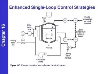
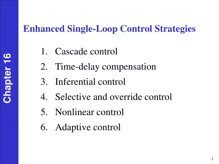
Enhanced Single-Loop Control Strategies. Cascade control Time-delay compensation Inferential control Selective and override control Nonlinear control Adaptive control. Chapter 16. Example: Cascade Control. Chapter 16. Chapter 16. Chapter 16. Cascade Control Distinguishing features:

E N D
Enhanced Single-Loop Control Strategies • Cascade control • Time-delay compensation • Inferential control • Selective and override control • Nonlinear control • Adaptive control Chapter 16
Example: Cascade Control Chapter 16
Cascade Control • Distinguishing features: • Two FB controllers but only a single control valve (or other final control element). • 2. Output signal of the "master" controller is the set-point for “slave" controller. • Two FB control loops are "nested" with the "slave" (or "secondary") control loop inside the "master" (or "primary") control loop. • Terminology: • slave vs. master • secondary vs. primary • inner vs. outer Chapter 16
Example 16.1 Consider the block diagram in Fig. 16.4 with the following transfer functions: Chapter 16
Example 16.2 Compare the set-point responses for a second-order process with a time delay (min) and without the delay. The transfer function is Assume and time constants in minutes. Use the following PI controllers. For min, while for min the controller gain must be reduced to meet stability requirements Chapter 16
Chapter 16 and If the process model is perfect and the disturbance is zero, then For this ideal case the controller responds to the error signal that would occur if not time were present. Assuming there is not model error the inner loop has the effective transfer function
Chapter 16 For no model error: By contrast, for conventional feedback control
Inferential Control • Problem: Controlled variable cannot be measured or has large sampling period. • Possible solutions: • Control a related variable (e.g., temperature instead of composition). • Inferential control: Control is based on an estimate of the controlled variable. • The estimate is based on available measurements. • Examples: empirical relation, Kalman filter • Modern term: soft sensor Chapter 16
Inferential Control with Fast and Slow Measured Variables Chapter 16
Selective Control Systems & Overrides • For every controlled variable, it is very desirable that there be at least one manipulated variable. • But for some applications, • NC > NM • where: • NC = number of controlled variables • NM = number of manipulated variables Chapter 16 • Solution: Use a selective control system or an override.
Low selector: Chapter 16 • High selector: • Median selector: • The output, Z, is the median of an odd number of inputs
Example: High Selector Control System Chapter 16 • multiple measurements • one controller • one final control element
Chapter 16 2 measurements, 2 controllers, 1 final control element
Overrides • An override is a special case of a selective control system • One of the inputs is a numerical value, a limit. • Used when it is desirable to limit the value of a signal (e.g., a controller output). • Override alternative for the sand/water slurry example? Chapter 16
Nonlinear Control Strategies • Most physical processes are nonlinear to some degree. Some are very nonlinear. Examples: pH, high purity distillation columns, chemical reactions with large heats of reaction. • However, linear control strategies (e.g., PID) can be effective if: 1. The nonlinearities are rather mild. or, 2. A highly nonlinear process usually operates over a narrow range of conditions. • For very nonlinear strategies, a nonlinear control strategy can provide significantly better control. • Two general classes of nonlinear control: 1. Enhancements of conventional, linear, feedback control 2. Model-based control strategies Reference: Henson & Seborg (Ed.), 1997 book. Chapter 16
Enhancements of Conventional Feedback Control We will consider three enhancements of conventional feedback control: • Nonlinear modifications of PID control • Nonlinear transformations of input or output variables • Controller parameter scheduling such as gain scheduling. Nonlinear Modifications of PID Control: Chapter 16 • One Example: nonlinear controller gain • Kc0 and a are constants, and e(t) is the error signal (e = ysp - y). • Also called, error squared controller. • Question: Why not use • Example: level control in surge vessels.
Nonlinear Transformations of Variables • Objective:Make the closed-loop system as linear as possible. (Why?) • Typical approach: transform an input or an output. Example: logarithmic transformation of a product composition in a high purity distillation column. (cf. McCabe-Thiele diagram) Chapter 16 • where x*D denotes the transformed distillate composition. • Related approach: Define u or y to be combinations of several variables, based on physical considerations. • Example: Continuous pH neutralization • CVs: pH and liquid level, h • MVs: acid and base flow rates, qA and qB • Conventional approach: single-loop controllers for pH and h. • Better approach: control pH by adjusting the ratio, qA/ qB, and control h by adjusting their sum. Thus, • u1 = qA/ qB and u2 =qA/ qB
Gain Scheduling • Objective:Make the closed-loop system as linear as possible. • Basic Idea: Adjust the controller gain based on current measurements of a “scheduling variable”, e.g., u, y, or some other variable. Chapter 16 • Note: Requires knowledge about how the process gain changes with this measured variable.
Examples of Gain Scheduling • Example 1. Titration curve for a strong acid-strong base neutralization. • Example 2. Once through boiler The open-loop step response are shown in Fig. 16.18 for two different feedwater flow rates. Fig. 16.18 Open-loop responses. Chapter 16 • Proposed control strategy: Vary controller setting with w, the fraction of full-scale (100%) flow. • Compare with the IMC controller settings for Model H in Table 12.1:
Adaptive Control • A general control strategy for control problems where the process or operating conditions can change significantly and unpredictably. Example: Catalyst decay, equipment fouling • Many different types of adaptive control strategies have been proposed. • Self-Tuning Control (STC): • A very well-known strategy and probably the most widely used adaptive control strategy. • Basic idea: STC is a model-based approach. As process conditions change, update the model parameters by using least squares estimation and recent u & y data. • Note: For predictable or measurable changes, use gain scheduling instead of adaptive control Reason: Gain scheduling is much easier to implement and less trouble prone. Chapter 16
Block Diagram for Self-Tuning Control Chapter 16