Download
1 / 37
370 likes | 507 Views
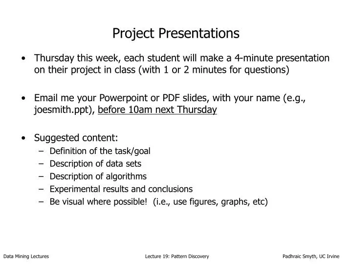
Project Presentations. Thursday this week, each student will make a 4-minute presentation on their project in class (with 1 or 2 minutes for questions) Email me your Powerpoint or PDF slides, with your name (e.g., joesmith.ppt), before 10am next Thursday Suggested content:

E N D
Project Presentations • Thursday this week, each student will make a 4-minute presentation on their project in class (with 1 or 2 minutes for questions) • Email me your Powerpoint or PDF slides, with your name (e.g., joesmith.ppt), before 10am next Thursday • Suggested content: • Definition of the task/goal • Description of data sets • Description of algorithms • Experimental results and conclusions • Be visual where possible! (i.e., use figures, graphs, etc) Data Mining Lectures Lecture 19: Pattern Discovery Padhraic Smyth, UC Irvine
Final Project Reports • Must be submitted as an email attachment (PDF, Word, etc) by 12 noon Tuesday next week • Use “ICS 278 final project report” in the subject line of your email • Report should be self-contained • Like a short technical paper • A reader should be able to repeat your results • Include details in appendices if necessary • Approximately 1 page of text per section (see next slide) • graphs/plots don’t count – include as many of these as you like. • Can re-use material from proposal and from midterm progress report if you wish Data Mining Lectures Lecture 19: Pattern Discovery Padhraic Smyth, UC Irvine
Suggested Outline of Final Project Report • Introduction: • Clear description of task/goals of the project • Motivation: why is this problem interesting and/or important? • Discussion of relevant literature • Summarize relevant aspects of prior published/related work • Technical approach • Data used in your project • Exploratory data analysis relevant to your task • Include as many of plots/graphs as you think are useful/relevant • Algorithms used in your project • Clear description of all algorithms used • Credit appropriate sources if you used other implementations • Experimental Results • Clear description of your experimental methodology • Detailed description of your results (graphs, tables, etc) • Discussion and Conclusions • What you learned from this project • Also: References and Appendices (if needed) Data Mining Lectures Lecture 19: Pattern Discovery Padhraic Smyth, UC Irvine
ICS 278: Data MiningLecture 19: Pattern Discovery Algorithms Padhraic Smyth Department of Information and Computer Science University of California, Irvine Data Mining Lectures Lecture 19: Pattern Discovery Padhraic Smyth, UC Irvine
Pattern-Based Algorithms • “Global” predictive and descriptive modeling • “global” models in the sense that they “cover” all of the data space • “Patterns” • More local structure, only describe certain aspects of the data • Examples: • A single small very dense cluster in input space • e.g., a new type of galaxy in astronomy data • An unusual set of outliers • e.g., indications of an anomalous event in time-series climate data • Associations or “rules” • If bread is purchased and wine is purchased then cheese is purchased with probability p • Motif-finding in sequences, e.g., • motifs in DNA sequences ~ noisy words in random background Data Mining Lectures Lecture 19: Pattern Discovery Padhraic Smyth, UC Irvine
General Ideas for Patterns • Many patterns can be described in the general form: • if condition 1 then condition 2 (with some certainty) • Probabilistic rules: If Age > 40 and education > college then income > $50k with probability p • “Bumps” If Age > 40 and education > college then mean income = $73k • if antecedent then consequent • if j then v • where j is generally some “box” in the input space • where v is a statement about a variable of interest, e.g., p(y | j ) or E [ y | j ] • Pattern support • “Support” = p( j ) or p(j , w ) • Fraction of points in input space where the condition applies • Often interested in patterns with larger support Data Mining Lectures Lecture 19: Pattern Discovery Padhraic Smyth, UC Irvine
How Interesting is a Pattern? • Note: “interestingness” is inherently subjective • Depends on what the data analyst already knows • Difficult to quantify prior knowledge • How interesting a pattern is, can be a function of • How surprising it is relative to prior knowledge? • How useful (actionable) it is? • This is a somewhat open research problem • In general pattern “interestingness” is difficult to quantify • => Use simple “surrogate” measures in practice Data Mining Lectures Lecture 19: Pattern Discovery Padhraic Smyth, UC Irvine
How Interesting is a Pattern? • Interestingness of a pattern • Measures how “interesting” the pattern j -> v is • Typical measures of interest • Conditional probability: p( v | j ) • Change in probability: | p( v | j ) - p( v ) | • “Lift” = p( v | j ) / p( v ) (also log of this) • Change in mean target response, e.g., E [y| j ]/E[y] Data Mining Lectures Lecture 19: Pattern Discovery Padhraic Smyth, UC Irvine
Pattern-Finding Algorithms • Typically… search a data set for the set of patterns that maximize some score function • Usually a function of both support and “interestingness” • E.g., • Association rules • Bump-hunting • Issues: • Huge combinatorial search space • How many patterns to return to the user • How to avoid problems with redundant patterns • Statistical issues • Even in random noise, if we search over a very large number of patterns, we are likely to find something that looks significant • This is known as “multiple hypothesis testing” in statistics • One approach that can help is to conduct randomization tests • e.g., for matrix data randomly permute the values in each column • Run pattern-discovery algorithm – resulting scores provide a “null distribution” • Ideally, also need a 2nd data set to validate patterns Data Mining Lectures Lecture 19: Pattern Discovery Padhraic Smyth, UC Irvine
Generic Pattern Finding Find patterns Task Representation pattern language f(support, interestingness) Score Function Search/Optimization greedy, branch-and-bound Data Management varies Models, Parameters list of K highest scoring patterns Data Mining Lectures Lecture 19: Pattern Discovery Padhraic Smyth, UC Irvine
Two Pattern Finding Algorithms • Bump-hunting: the PRIM algorithm Bump Hunting in High Dimensional Data J. H. Friedman & N. I. Fisher Statistics and Computing, 2000 • Market basket data: association rule algorithms Data Mining Lectures Lecture 19: Pattern Discovery Padhraic Smyth, UC Irvine
“Bump-Hunting” (PRIM) algorithm • Patient Rule Induction Method (PRIM) • Friedman and Fisher, 2000 • Addresses “bump-hunting” problem: • Assume we have a target variable Y • Y could be real-valued or a binary class variable • And we have p “input” variables • We want to find “boxes” j in input space where E[Y| j ] >> E[Y] • or where E[Y| j ] << E[Y] , i.e., “data holes” • A box j is a “conjunctive sentence”, e.g., if Age < 22 and occupation = student Example of a “box pattern” if Age > 30 and education > bachelor then E[income | j ] = $120k Data Mining Lectures Lecture 19: Pattern Discovery Padhraic Smyth, UC Irvine
“Bump Hunting”: Extrema Regions for Target f(x) • let Sj be set of all possible values for input variable xj • entire input domain is S = S1 S2 … Sd • goal: find subregion R S for which • mR = avg xR f(x) >> m • where m = f(x) p(x) dx (target mean, over all inputs) • subregion size as fraction of full space (“support”): • R = xR p(x) dx • tradeoff between mR and R (increase R => reduce mR) ... • sample-based estimates used in practice: • R = (1/n) XiR 1(XiR), yavgR = 1/(nR) XiR yi • note: mR is true quantity of interest, not yavgR Data Mining Lectures Lecture 19: Pattern Discovery Padhraic Smyth, UC Irvine
Greedy Covering • a generic greedy covering algorithm • first box B1 induced from entire data set • second box B2 induced from data not covered by B1 • … BK induced from remaining data {yi,Xi | Xi j=1…K-1 Bj} • do until either: • estimated target mean f(x) in Bk becomes too small • yavgK = avg[yi | Xi Bk &Xi j=1…K-1 Bj] < = (1/n) ni=1 yi • support of Bk becomes too small • K = (1/n) i=1…n 1(Xi Bk &Xi j=1…K-1 Bj) • then select set of boxes R = j Bj for some threshold • for which each yavgj >someyavgthreshold or • yield largest yavgR for which R =i i some threshold Data Mining Lectures Lecture 19: Pattern Discovery Padhraic Smyth, UC Irvine
PRIM algorithm • PRIM uses “patient greedy search” on individual variables • Start with all training data and maximal box • Repeat until minimal box (e.g., minimal support or n<10) • Shrink box by compressing one face of the box • For each variable in input space • “Peel” off a proportion of observations to optimize E[y |new box], • typical =0.05 or =0.1 • Now “expand” the box if E[y|box] can be increased (“pasting”) • Yields a sequence of boxes • Use cross-validation (on E[y|box]) to select the best box • Remove box from training data, then repeat process Data Mining Lectures Lecture 19: Pattern Discovery Padhraic Smyth, UC Irvine
Data Mining Lectures Lecture 19: Pattern Discovery Padhraic Smyth, UC Irvine
Comments on PRIM • Works one variable at a time • So time-complexity is similar to tree algorithms, i.e., • Linear in p, and n log n for sorting • Nominal variables • Can peel/paste on single values, subsets, negations, etc • Similar in some sense to CART….but • More “patient” in search (removes only small fraction of data at each step) • Useful for finding “pockets” in the input space with high-response • e.g., marketing data: small groups of consumers who spend much more on a given product than the average consumer • Medical data: patients with specific demographics whose response to a drug is much better than the average patient Data Mining Lectures Lecture 19: Pattern Discovery Padhraic Smyth, UC Irvine
Marketing Data Example (n=9409, p=502) • freq air travel: y=num flights/yr, global mean(y)=1.7 • B1: mean(y1)=4.2, 1=0.08 (8% market seg) • education >= 16 yrs; income > $50K & missing • occupation in {professional/manager, sales, homemaker} • number of children (<18) in home <= 1 • B2: mean(y2)=3.2, 2=0.07 (~2x global mean) • education > 12 yrs & missing • income > $30K & missing; 18 < age < 54 • married / dual income in {single, married-one-income} • these boxes intuitive: nothing really surprising ... Data Mining Lectures Lecture 19: Pattern Discovery Padhraic Smyth, UC Irvine
Pattern Finding Algorithms • Bump-hunting: the PRIM algorithm • Market basket data: association rule algorithms Data Mining Lectures Lecture 19: Pattern Discovery Padhraic Smyth, UC Irvine
Items x x x x x x x x Transactions x x x x x x Transaction Data and Market Baskets • Supermarket example: (Srikant and Agrawal, 1997) • #items = 50,000, #transactions = 1.5 million • Data sets are typically very sparse x x x x x x x Data Mining Lectures Lecture 19: Pattern Discovery Padhraic Smyth, UC Irvine
Market Basket Analysis • given: a (huge) “transactions” database • each transaction representing basket for 1 customer visit • each transaction containing set of items (“itemset”) • finite set of (boolean) items (e.g. wine, cheese, diaper, beer, …) • Association rules • classically used on supermarket transaction databases • associations: Trader Joe’s customers frequently buy wine & cheese • rule: “people who buy wine also buy cheese 60% of time” • infamous “beer & diapers” example: • “in evening hours, beer and diapers often purchased together” • generalize to many other problems, e.g.: • baskets = documents, items = words • baskets = WWW pages, items = links Data Mining Lectures Lecture 19: Pattern Discovery Padhraic Smyth, UC Irvine
Market Basket Analysis: Complexity • usually transaction DB too huge to fit in RAM • common sizes: • number of transactions: 105 to 108 (hundreds of millions) • number of items: 102 to 106 (hundreds to millions) • entire DB needs to be examined • usually very sparse • e.g. ~ 0.1% chance of buying random item • subsampling often a useful trick in DM, but • here, subsampling could easily miss the (rare) interesting patterns • thus, runtime dominated by disk read times • motivates focus on minimizing number of disk scans Data Mining Lectures Lecture 19: Pattern Discovery Padhraic Smyth, UC Irvine
Association Rules: Problem Definition • given: set I of items, set T transactions, t T, t I • Itemset Z = a set of items (any subset of I) • support count(Z) = num transactions containing Z • given any itemset Z I, (Z) = | { t | t T, Z t } | • association rule: • R=“X Y [s,c]”, X,Y I, XY= • support: • s(R) = s(XY) = (XY)/|T| = p(XY) • confidence: • c(R) = s(XY) / s(X) = (XY) / (X) = = p(X | Y) • goal: find all R such that • s(R) given minsup • c(R) given minconf Data Mining Lectures Lecture 19: Pattern Discovery Padhraic Smyth, UC Irvine
Comments on Association Rules • association rule: R=“X Y [s,c]” • Strictly speaking these are not “rules” • i.e., we could have “wine => cheese” and “cheese => wine” • correlation is not causation • The space of all possible rules is enormous • O( 2p ) where p = the number of different items • Will need some form of combinatorial search algorithm • How are thresholds minsup and minconf selected? • Not that easy to know ahead of time how to select these Data Mining Lectures Lecture 19: Pattern Discovery Padhraic Smyth, UC Irvine
Example • simple example transaction database (|T|=4): • Transaction1 = {A,B,C} • Transaction2 = {A,C} • Transaction3 = {A,D} • Transaction4 = {B,E,F} • with minsup=50%, minconf=50%: • R1: A --> C [s=50%, c=66.6%] • s(R1) = s({A,C}) , c(R1) = s({A,C})/s({A}) = 2/3 • R2: C --> A [s=50%, c=100%] • s(R2) = s({A,C}), c(R2) = s({A,C})/s({C}) = 2/2 s({A}) = 3/4 = 75% s({B}) = 2/4 = 50% s({C}) = 2/4 = 50% s({A,C}) = 2/4 = 50% Data Mining Lectures Lecture 19: Pattern Discovery Padhraic Smyth, UC Irvine
Finding Association Rules • two steps: • step 1: find all “frequent” itemsets (F) • F = {Z | s(Z) minsup} (e.g. Z={a,b,c,d,e}) • step 2: find all rules R: X --> Y such that: • X Y F and X Y= (e.g. R: {a,b,c} --> {d,e}) • s(R) minsup and c(R) minconf • step 1’s time-complexity typically >> step 2’s • step 2 need not scan the data (s(X),s(Y) all cached in step 1) • search space is exponential in |I|, filters choices for step 2 • so, most work focuses on fast frequent itemset generation • step 1 never filters viable candidates for step 2 Data Mining Lectures Lecture 19: Pattern Discovery Padhraic Smyth, UC Irvine
Finding Frequent Itemsets • frequent itemsets: {Z | s(Z)>minsup} • “Apriori (monotonicity) Principle”: s(X) s(XY) • any subset of a frequent itemset must be frequent • finding frequent itemsets: • bottom-up approach: • do level-wise, for k=1 … |I| • k=1: find frequent singletons • k=2: find frequent pairs (often most costly) • step k.1: find size-k itemset candidates from the freq size-(k-1)’s of prev level • step k.2 prune candidates Z for which s(Z)<minsup • each level requires a single scan over all the transaction data • computes support counts (Z) = | { t | t T, Z t } for all size-k Z candidates s({A}) = 3/4 = 75% s({B}) = 2/4 = 50% s({C}) = 2/4 = 50% s({A,C}) = 2/4 = 50% Data Mining Lectures Lecture 19: Pattern Discovery Padhraic Smyth, UC Irvine
bottleneck: Apriori Example (minsup=2) itemset {1,2} {1,3} {1,5} {2,3} {2,5} {3,5} C2 F1 C1 transactions T {1,3,4} {2,3,5} {1,2,3,5} {2,5} itemset sup {1} 2 {2} 3 {3} 3 {4} 1 {5} 3 itemset sup {1} 2 {2} 3 {3} 3 {5} 3 gen count (scan T) filter count (scan T) F3 itemset sup {2,3,5} 2 C2 C3 knows can avoid gen {1,2,3} (and {1,3,5}) apriori, without counting, because {1,2} ({1,5}) not freq itemset sup {1,2} 1 {1,3} 2 {1,5} 1 {2,3} 2 {2,5} 3 {3,5} 2 F2 filter itemset sup {1,3} 2 {2,3} 2 {2,5} 3 {3,5} 2 C3 itemset sup {2,3,5} 2 notice how |C3| << |C2| C3 filter itemset {2,3,5} count (scan T) gen Data Mining Lectures Lecture 19: Pattern Discovery Padhraic Smyth, UC Irvine
Data Mining Lectures Lecture 19: Pattern Discovery Padhraic Smyth, UC Irvine
Problems with Association Rules • Consider 4 highly correlated items A, B, C, D • Say p(subset i|subset j) > minconf for all possible pairs of disjoint subsets • And p(subset i subset j) > minsup • How many possible rules? • E.g., A->B, [A,B]=>C, [A,C]=>B, [B,C]=>A • All possible combinations: 4 x 23 • In general for K such items, K x 2K-1 rules • For highly correlated items there is a combinatorial explosion of redundant rules • In practice this makes interpretation of association rule results difficult Data Mining Lectures Lecture 19: Pattern Discovery Padhraic Smyth, UC Irvine
References on Association Rules • Chapter 13 in text (Sections 13.1 to 13.5) • Early papers: • R. Agrawal and R. Srikant, Fast algorithms for mining association rules, in Proceedings of VLDB 1994, pp.487-499, 1994. • R. Agrawal et al. Fast discovery of association rules, in Advances in Knowledge Discovery and Data Mining, AAAI/MIT Press, 1996. • More recent: • Good review in Chapter 6 of Data Mining: Concepts and Techniques, J. Han and M. Kamber, Morgan Kaufmann, 2001. • J. Han, J. Pei, and Y. Yin, Mining frequent patterns without candidate generation, Proceedings of SIGMOD 2000, pages 1-12. • Z. Zheng, R. Kohavi, and L. Mason, Real World Performance of Association Rule Algorithms, Proceedings of KDD 2001 Data Mining Lectures Lecture 19: Pattern Discovery Padhraic Smyth, UC Irvine
Study on Association Rule Algorithms • Z. Zheng, R. Kohavi, and L. Mason, Real World Performance of Association Rule Algorithms, Proceedings of KDD 2001 • Evaluated a variety of association rule algorithms • Used both real and simulated transaction data sets • Typical real data set from Web commerce: • Number of transactions = 500k • Number of items = 3k • Maximum transaction size = 200 • Average transaction size = 5.0 Data Mining Lectures Lecture 19: Pattern Discovery Padhraic Smyth, UC Irvine
Study on Association Rule Algorithms • Conclusions: • Very narrow range of minsup yields interesting rules • Minsup too small => too many rules • Minsup too large => misses potentially interesting patterns • Superexponential growth of rules on real-world data • Real-world data is different to simulated transaction data used in research papers, e.g., • Simulated transaction sizes have a mode away from 1 • Real transaction sizes have a mode at 1 and are highly skewed • Speed-up improvements demonstrated on artificial data did not generalize to real transaction data Data Mining Lectures Lecture 19: Pattern Discovery Padhraic Smyth, UC Irvine
Beyond Binary Market Baskets • counts (vs yes/no) • e.g. “3 wines” vs “wine” • quantitative (non-binary) item variables • popular: discretize real variable into k binary variables • e.g. {age=[30:39],incomeK=[42:48]} buys_PC • Item hierachies • Common in practice, e.g., clothing -> shirts -> men’s shirts, etc • Can learn rules that generalize across the hierarchy • mining sequential associations/patterns and rules • e.g. {1@0,2@5} 4@15 Data Mining Lectures Lecture 19: Pattern Discovery Padhraic Smyth, UC Irvine
Association Rule Finding Find association rules Task Representation [A and B] => C P(A,B,C) > minsup, P(C|A, B) > minconf Score Function Breadth-first candidate generation Search/Optimization Data Management Linear scans Models, Parameters list of all rules satisfying thresholds Data Mining Lectures Lecture 19: Pattern Discovery Padhraic Smyth, UC Irvine
Bump Hunting (PRIM) Find high score bumps Task Representation [A,B] => E[y|A,B] > E[y] Score Function E[y|A,B] and p(A,B) Search/Optimization Greedy search Data Management None Models, Parameters Set of “boxes” Data Mining Lectures Lecture 19: Pattern Discovery Padhraic Smyth, UC Irvine
Summary • Pattern finding • An interesting and challenging problem • How to search for interesting/unusual “regions” of a high-dimensional space • Two main problems • Combinatorial search • How to define “interesting” (this is the harder problem) • Two examples of algorithms • PRIM for bump-hunting • Apriori for association rule mining • Many open problems in this research area (room for new ideas!) Data Mining Lectures Lecture 19: Pattern Discovery Padhraic Smyth, UC Irvine