Biostatistics course Part 12 Association between two categorical variables

1. Biostatistics coursePart 12Association between two categorical variables Dr. Sc. Nicolas Padilla Raygoza Department of Nursing and Obstetrics Division Health Sciences and Engineering Campus Celaya-Salvatierra University of Guanajuato, Mexico

2. Biosketch • Medical Doctor by University Autonomous of Guadalajara. • Pediatrician by the Mexican Council of Certification on Pediatrics. • Postgraduate Diploma on Epidemiology, London School of Hygiene and Tropical Medicine, University of London. • Master Sciences with aim in Epidemiology, Atlantic International University. • Doctorate Sciences with aim in Epidemiology, Atlantic International University. • Associated Professor B, Department of Nursing and Obstetrics, Division of Health Sciences, University of Guanajuato Campus Celaya Salvatierra. • padillawarm@gmail.com

3. Competencies • The reader will analyze the relationship between two categorical variables with two or more categories. • He (she) will apply the Chi-squared test. • He (she) will know the Chi-squared test for trends and when apply it.

4. Introduction • In part three, we learned how to tabulate a frequency distribution for a categorical variable. This tab shows how individuals are distributed in each category of a variable. • For example, in a rural community in Celaya, a randomized sample of 200 people were asked about their level of socioeconomic status.

5. Introduction • The table shows the distribution of individuals in each category Socioeconomic Index Level (SEIL).

6. Introduction • When we examine the relationship between two categorical variables, tabulated one against other. • This is a two way table or cross-tabulation.

7. Interpretation of a two ways table • There is an association between two categorical variables, if the distribution of a variable varies according to the value of the other. • The question we are interested in is: • Is the level of SEIL varies by place of residence? • To answer this question we need to assess a cross-tabulation

8. Interpretation of a two ways table • To compare the distributions in the table, we need to consider the percentages. To answer the question of interest, what should we consider the percentages of column or row? Place of residence

9. Expected frequencies • If the null hypothesis is true, there is no association between SEIL and area of residence, the percentages for each level of SEIL in each area, should be the same as the column of percentages in the total column.

10. Example of expected frequencies • The percentage of people in low SEIL in the total sample is 50 (25%). • If the null hypothesis is true, we should expect that 25% of people in the place of residence, Center, with low SEIL, are: 25% of 96 = 24

11. Interpretation of a two ways table Place of residence

12. Example of expected frequencies • If there are no differences in the distribution of SEIL by places of residence, we should expect that the percentage of people with low SEIL is the same in each place of residence. • Note that the expected frequencies do not have to be integers. • Using the totals of columns and rows, we can calculate the expected number in each cell

13. Chi-squared test • Expected frequencies are those that we should expect if the null hypothesis were true. • To test the null hypothesis, we must compare the expected frequencies with observed frequencies, using the following formula. (O – E)2 X2=Σ-------------- E

14. Chi-squared test • From the formula we can see that: • If there is a significant difference between the observed and expected values, X2 will be great • If there is a small difference between the observed and expected values, X2 will be small. • If X2 is large, suggesting that data do not support the null hypothesis because the observed values are not what we expect under the null hypothesis. • If X2 is small, the data suggests that support from the null hypothesis that the observed values are similar to those expected under the null hypothesis.

15. Chi-squared test Place of residence

16. Chi-squared test

17. Chi-squared test in 2 x 2 tables • When both variables are binary, the cross-tabulation table becomes a 2 x 2. • The X2 test was applied in the same way as for a larger table.

18. Example • There was a study of the bacteriological efficacy of clarithromycin vs penicillin, in acute pharyngotonsillitis in children by Streptococcus Beta Haemolytic Group A. • The results are shown below

19. Example • To use Chi-squared test, we should point the null hypothesis; in this case, it should be: • There are not differences between bacteriological efficacy between the two treatments, against Streptococcus Beta Hemolytic Group A. • To test the null hypothesis, first we should calculate the expected numbers in each cell from the table.

20. Example

21. A quickly formulae for 2 x 2 tables • X2 can be calculate using the observed frequencies in a table and marginal totals. • If we labeled the cells and marginal totals as follow: X2=(ad – bc)2 x N /(a+b) (c+d) (a+c) (b+d)

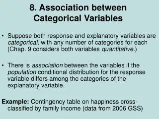
22. Trend test in 2 x c tables • We had use Chi-squared test to evaluate if two categorical variables are associated between them in the population. • When one variable is binary and another is ordered categorical (ordinal), we can be interested in to comprobe if their association follow a trend.

23. Trend test in 2 x c tables SEIL

24. Trend test in 2 x c tables • To calculate this test, assign a numerical score to each socioeconomic group. SEIL

25. Chi-squared test trends • We conducted a chi-square test for trend, when we assess whether a binary variable, varies linearly through the levels of another variable, to assess whether there is a dose-response effect. • The null hypothesis for this test is that the mean scores in the two groups (the binary variable) are the same. • Thus, the Chi square test becomes a test comparing two means by this is with only one degree of freedom.

26. Chi-squared test for trends _ _ (X (Yes) – X (No))2 X2 = ------------------- = S2 (1/n1 + 1/n2) _ X (Yes) = mean of score from hypertension group _ X (No) = mean of score from non-hypertension group n1 total of people in hypertension group n2 total of people in non-hypertension group s= standard deviation for overall scores from both groups

27. Validity of Chi-squared tests • Chi square tests that we reviewed are based on the assumption that the test statistic follows approximately the distribution of X2. • This is reasonable for large samples but for the small one should use the following guidelines: • For 2 x 2 tables • If the total sample size is> 40, then X2 can be used. • If n is between 20 and 40, and the smallest expected value is 5, X2 can be used. • Otherwise, use the exact value of Fisher. • 2 x c tables • The X2 test is valid if not more than 20% of expected values is less than 5 and none is less than 1.

28. Bibliografy • 1.- Last JM. A dictionary of epidemiology. New York, 4ª ed. Oxford University Press, 2001:173. • 2.- Kirkwood BR. Essentials of medical ststistics. Oxford, Blackwell Science, 1988: 1-4. • 3.- Altman DG. Practical statistics for medical research. Boca Ratón, Chapman & Hall/ CRC; 1991: 1-9.