Download
1 / 14
140 likes | 219 Views
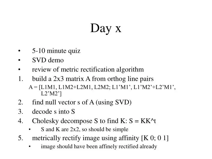
Day x. 5-10 minute quiz SVD demo review of metric rectification algorithm build a 2x3 matrix A from orthog line pairs A = [L1M1, L1M2+L2M1, L2M2; L1’M1’, L1’M2’+L2’M1’, L2’M2’] find null vector s of A (using SVD) decode s into S Cholesky decompose S to find K: S = KK^t

E N D
Day x • 5-10 minute quiz • SVD demo • review of metric rectification algorithm • build a 2x3 matrix A from orthog line pairs A = [L1M1, L1M2+L2M1, L2M2; L1’M1’, L1’M2’+L2’M1’, L2’M2’] • find null vector s of A (using SVD) • decode s into S • Cholesky decompose S to find K: S = KK^t • S and K are 2x2, so should be simple • metrically rectify image using affinity [K 0; 0 1] • image should have been affinely rectified already
Epipolar geometry HZ 9.1 Fundamental matrix HZ 9.2 normalized 8-pt alg for F HZ 11.2 7-point algorithm Camera from F Structure computation Alg 12.1, HZ318
Linear constraints on F • let x = (x,y,1) and x’ = (x’,y’,1) be a point correspondence between 2 images, and let F be the fundamental matrix of the images • we know that the point pair satisfies x’ F x = 0 • this generates a linear constraint on the entries of F = (fij): • x’xf11 + x’yf12 + x’f13 + y’xf21 + ... + f33 = 0 • (x’x, x’y, x’, y’x, y’y, y’, x, y, 1) f = 0 • where f = (f11,12,...,f33) encodes F in row-major order • each point correspondence (xi,xi’) yields a row (xi’xi, xi’yi, xi’, yi’xi, yi’yi, yi’, xi, yi, 1) • collect n rows (x’x, x’y, x’, y’x, y’y, y’, x, y, 1) into nx9 matrix A • F is found as the solution of Af = 0 • HZ279
Solving Af=0 • if data is exact and rank(A) is exactly 8, then f is found as the null vector of A • in a perfect world, Af=0 has a solution • recall: use SVD (and last column of V) to compute the null vector • if data is noisy and rank(A) = 9, then f is found as a least squares solution • min ||Af|| • SVD, use last column of V • just like in the DLT algorithm • HZ280
The singularity constraint without with • force F to be singular • we know the correct F is singular (see above) • we need F to be singular, since the epipoles are computed using its null space • due to noise, the computed F will not be singular • how? use another SVD! • let F = UDV^t where D = diag(r,s,t) with r>=s>=t • let F’ = UD’V^t where D’ = diag(r,s,0) • this is guaranteed to be singular since det(F’) = 0 • HZ280-281
Preconditioning • recall preconditioning in DLT algorithm • apply it in 8 point algorithm for F too • before creating A (as in Af=0) from the point correspondences, normalize the points • centroid to origin translation + scaling to \sqrt 2 average distance • also called root mean square (RMS) scaling • let xi Txi and xi’ T’xi’ be the transformation matrices • denormalize via F T’t F T after finding F (i.e., after enforcing the singularity constraint) • shampoo? • HZ282
Normalized 8 point algorithm • basically 2 SVD’s, the first to find F and the second to refine it • the fodder for the SVD’s is a matrix built from the point correspondences • SIFT: find a set of at least 8 point correspondences (xi,xi’) • precondition each pointset {xi} and {xi’} independently (with T and T’) • [solve for F as a null vector f] • build nx9 matrix A from x^t F x = 0 constraints, n>=8 • compute SVD of A: A = U1 D V1^t • f = row-major encoding of F = null vector of A = last column of V1 • [impose singularity constraint] • compute SVD of F: F = U2 D V2t • replace F by U2 diag(d11,d22,0) V2t • postcondition: replace F by T’t F T • SPASSP (SIFT, precondition, A, SVD for f, SVD for singularity, postcondition) • HZ282, Alg 11.1
7-point algorithm • F has 8dof so we need 8 constraints • but the singularity constraint (det F = 0) can act as one of the 8 constraints • hence, only need 7 constraints from point correspondences • build 7x9 matrix A (as above) • the 2D null space of Af=0 is spanned by the last 2 columns of V in the SVD of A • let v1 and v2 be the last 2 columns of V • the vector family f(t) = (1-t)v1 + tv2 yields a matrix family F(t) = (1-t)F1 + tF2 • now solve det (F(t)) = 0 for t • since det(F(t)) is a cubic polynomial in t, it has 1 or 3 real roots • hence, this algorithm yields 1 or 3 solutions for F • HZ281
More than one solution for F • degeneracy: 3 solutions if the camera centers and 3D points Xi (from which the point pairs (xi,xi’)) all lie on a ‘critical surface’ • critical surface can be two planes, cone, cylinder or hyperboloid of one sheet (N.B. always a ruled quadric) • this is quite likely in the 7-point algorithm: 7 points and 2 camera centers always lie on some quadric, since 9 points define a quadric • the only question is whether the quadric is ruled or not (ellipsoid, hyperboloid of one sheet) • beware of all points in the same plane, or identical camera centers • this will yield a 2d family of family of fundamental matrices! • HZ296
Iterative optimization • an even better approximation to F can be found using an iterative method, bootstrapping from the 7-point or 8-point solutions • based on the idea of searching only for singular matrices that minimize ||Af|| • rather than separating out the singularity constraint in a later stage • requires the epipole, which we do not know, so it leads to an iterative process • guess F, compute associated e, compute new F, iterate • this goes beyond our scope here: we’ll talk about it in seminar • techniques: 2 SVD’s (HZ595 minimizations) and Levenberg-Marquardt algorithm (HZ600): Algorithm 11.2, HZ284 • there is also a gold standard algorithm that involves even more computation: Algorithm 11.3, HZ285 • HZ282-285; HZ595,600
Which algorithm is best? • an algorithm for computing F may be evaluated by computing the distance of a point xi’ from the computed epipolar line Fxi • conclusions from HZ experiments (Figure 11.3): • normalized 8-pt algorithm performs just fine • use more than 8 points: error is reduced up to about 15 points, then starts leveling off • 8-point with 15 points is better than more elaborate algorithms on 8 points • add RANSAC estimation for added robustness (Alg 11.4) • note that we are computing F with no user interaction • HZ288-291
Adding RANSAC without with • avoids outlier contamination • SIFT will have plenty of outliers • HZ290-291
Don’t use line correspondences • fascinating: line correspondences offer no information in 2 images! • reason: 2 points backproject to 2 lines, which must intersect if the points are corresponding • this adds a constraint, since 2 lines in 3-space do not intersect in general • however, 2 lines backproject to 2 planes, and 2 planes always intersect, so there is no added constraint • line correspondences do become useful in 3 views: see trifocal tensors • HZ294
But curve correspondences are useful • shared tangency at epipolar lines can be leveraged to add a constraint • corresponding curves in the 2 images must be tangent to the corresponding epipolar lines • see Exercises (ii) and (iii) at end of Chapter 11 • tangency again: we will explore later • HZ295, 309