Download

1 / 58
890 likes | 1.57k Views
LOG-LINEAR MODEL FOR CONTIGENCY TABLES. Mohd Tahir Ismail School of Mathematical Sciences Universiti Sains Malaysia. The Log-linear Analysis procedure analyzes the frequency counts of observations falling into each cross- classification category in a cross tabulation or a contingency table

E N D
LOG-LINEAR MODEL FOR CONTIGENCY TABLES MohdTahir Ismail School of Mathematical Sciences UniversitiSains Malaysia
The Log-linear Analysis procedure analyzes the frequency counts of observations falling into each cross- classification category in a cross tabulation or a contingency table • Each cross-classification in the table constitutes a cell, and each categorical variable is called a factor • The ultimate goal of fitting a log-linear model is to estimate parameters that describe the relationships between categorical variables INTRODUCTION
Specifically, for a set of categorical variables, log-linear models treat all variables as response variables by modelling the cell counts for all combinations of the levels of the categorical variables included in the model • Therefore, fitting a log-linear model is appropriate when all of the variables are categorical in nature and a researcher is interested in understanding how a count within a particular cell of the contingency table depends on the different levels of the categorical variables that define that particular cell INTRODUCTION
Logistic regression is concerned with modeling a single binary valued response variable as a function of covariates • There are many situations, however, where several factors simultaneously interact with each other in a multivariate manner and the cause and effect relationship is unclear • Log-linear models were developed to analyze this type of data • Logistic regression is a special case of log-linear models INTRODUCTION
In general, the number of parameters in a log-linear model depends on the number of categories of the variables of interest • More specifically, in any log-linear model the effect of a categorical variable with a total of C categories requires (C – 1) unique parameters • For example, if variable X is gender (with two categories), then C=2 and only one predictor, thus one parameter, is needed to model the effect of X. Coding of Variables Log-linear Models
One of the simplest and most intuitive ways to code categorical variables is called “dummy coding.” • When dummy coding is used, the last category of the variable is used as a reference category. • Therefore, the parameter associated with the last category is set to zero, and each of the remaining parameters of the model is interpreted relative to the last category. Coding of Variables Log-linear Models
Instead of representing the parameter associated with the ith variable (Xi) as ,in log-linear models this parameter is represented by the Greek letter lambda, • ,with the variable indicated in the superscript and the (dummy-coded) indicator of the variable in the subscript • For example, if the variable X has a total of I categories (i =1, 2, …, I), is the parameter associated with the i-th indicator (dummy variable) for X Notation of Variables
An investigator intend to assess the contribution that overweight and smoking cause to coronary artery disease. Data are collected based on ECG reading, BMI and whether smoking or not for a sample of 188 people Using SPSS-Example
categorical data • each categorical variable is called a factor • every case should fall into only one cross-classification category • all expected frequencies should be greater than 1, and not more than 20% should be less than 5. • 1. collapse the data across one of the variables • 2. collapse levels of one of the variables • 3. collect more data • 4. accept loss of power • 5. add a constant (0.5) to all cells of the table Check Assumptions
From the Model Selection box, Select any variables that you want to include in the analysis by selecting them with the mouse
If you click on Model button then this will open a dialog box, check...
Clicking on Options opens another dialog box. There are few options to play around with really (the default options are fine) The only two things you can select are Parameter estimates, which will produce a table of parameter estimates for each effect and for an Association table, which will produce chi-square statistics for all of the effects in the model
The first table tells us that we have 188 cases. SPSS then lists all of the factors in the model and the number of levels they have Output from Log-linear Analysis
The second table gives us the observed and expected counts for each of the combinations of categories in our model.
The final bit of this initial output gives us two goodness-of-fit. In this context these tests are testing the hypothesis that the frequencies predicted by the model (the expected frequencies) are significantly different from the actual frequencies in our data (the observed frequencies) The next part of the output tells us something about which components of the model can be removed.
The likelihood ratio chi-square with no parameters and only the mean is 49.596. The value for the first order effect is 31.093. The difference 49.596 − 31.093 =18.503 is displayed on the first line of the next table. The difference is a measure of how much the model improves when first order effects are included. The significantly small P value (0.0000) means that the hypothesis of first order effect being zero is rejected. In other words there is a first order effect.
Similar reasoning is applied now to the question of second order effect. The addition of a second order effect improves the likelihood ratio chi-square by 28.656. This is also significant. But the addition of a third order term does not help. The P value is not significant. In log-linear analysis the change in the value of the likelihood ratio chi-square statistic when terms are removed (or added) from the model is an indicator of their contribution. We saw this in multiple linear regression with regard to R2. The difference is that in linear regression large values of R2 are associated with good models. Opposite is the case with log-linear analysis. Small values of likelihood ratio chi-square mean a good model.
This simply breaks down the previous table that we’ve just looked at into its component parts. So, for example, although we know from the previous output that removing all of the two-way interactions significantly affects the model, we don’t know which of the two-way interactions is having the effect
Keep in mind, though, that regardless of the partial association test, one must retain even nonsignificant lower-order terms if they are components of a significant higher-order term which is to be retained in the model. • Thus in the example above, one would retain ECG and BMI even though they are non-significant because they are terms in the two significant two-way interactions, ECG*BMI and BMI*Smoke • Thus the partial associations test suggest dropping only the ECG*Smoke interaction.
The output above lists each main and interaction effect in the hierarchy of all effects generated by the highest-order interaction in the set of factors the researcher enters. This not-printed parameter estimate for the left-out category is the negative of the sum of the printed parameter estimates (since the estimates must add to 0).
The purpose here is to find the unsaturated model that would provide the best fit to the data. This is done by checking that the model currently being tested does not give a worse fit than its predecessor As a first step the procedure commences with the most complex model. In our case it is BMI * ECG * SMOKE. Its elimination produces a chi-square change of 1.389, which has an associated significance level of 0.2386. Since it is greater than the criterion level of 0.05, it is removed. The procedure moves on to the next hierarchical level described under step 1. All 2 – way interactions between the three variables are being tested. Removal of ECG*BMI will produce a large change of 14.601 in the likelihood ratio chi-square. The P value for that is highly significant (prob = 0.0000). The smallest change (of 2.406 ) is related to the ECG * SMOKE interaction. This is removed next. And the procedure continues until the final model which gives the second order interactions of ECG * BMI and BMI * SMOKE.
We conclude that being overweight and smoking have each a significant association with an abnormal cardiogram. However, in this particular group of subjects being overweight is more harmful.
Estimate the model using Loglinear-General to print parameter estimates
From the General box, Select any variables that you want to include in the analysis by selecting them with the mouse
Click the Model button to define the model. We are interested in a model with fewer terms and then we must click the Custom button.
Recall that the best model generated by the Model Selection procedure was the full factorial model minus the ECG*Smoke. The goodness of fit tests show that the fit is perfect: both goodness of fit statistics are not significant. The Output