Download
1 / 34
340 likes | 348 Views
Coupling Chemical Transport Model Source Attributions with Positive Matrix Factorization: Application to two IMPROVE sites impacted by wildfires. Sturtz et. al. 2014 ATMS 790 seminar Ashley Pierce. Outline. Background Source Apportionment Positive Matrix Factorization (PMF)

E N D
Coupling Chemical Transport Model Source Attributions with Positive Matrix Factorization: Application to two IMPROVE sites impacted by wildfires Sturtz et. al. 2014 ATMS 790 seminar Ashley Pierce
Outline • Background • Source Apportionment • Positive Matrix Factorization (PMF) • Chemical Transport Model (CTM) • Hybrid • The study • Model comparison and evaluation • Implications
Background • Particulate matter (PM2.5): mixture of small particles and liquid drops • Aerosol: PM suspended in a gas (e.g. air) • Volatile Organic Compounds (VOCs): variety of chemicals (benzene, isoprene) • Secondary Organic Aerosols (SOA) • Carbonaceous aerosols – major component of fine particulate mass • IMPROVE: Interagency Monitoring of Protected Visual Environments (1985) • National Ambient Air Quality Standards (NAAQS)
Source Apportionment Meteorology Primary & secondary pollutants Transport, transformation, & removal processes Transport, transformation, & removal processes CTM Primary & secondary pollutants Primary pollutants PMF Emission Source (Anthropogenic combustion, biomass burning, biogenic emissions from plants) Receptor Affected site/organism or measurement area • Source-Receptor relationship: determining the role of meteorology and physical/chemical effects linking source emissions to receptor concentrations • Source profiles: the experimentally determined unique proportion of species concentrations • (or speciated PM or speciated aerosol) from a source • Ex. Biomass burning – OC, EC, levoglucosan • Feature: A factor profile (source factor) unique proportion of speciated aerosols determined by the PMF analysis
Particulate carbon • Fossil carbon: coal, oil, gas fuels • Biogenic carbon: biomass burning, meat cooking, Secondary organic aerosols (SOAs) • Upper bound for biomass burning contribution
More volatile, lower light absorption Higher light absorption http://www.lucci.lu.se/wp1_projects.html
Importance • Adversely affect health, contribute to haze, affect radiation balance • Biogenic sources of carbonaceous aerosols • 80-100% of fine particulate carbon in rural areas • ~50% in some urban areas • Carbonaceous species often largest contributor to haze and PM2.5 • Smoke thought to be large contributor (W and SE U.S.) • Difficult to apportion smoke from other emissions or between smoke types • >50% of smoke particulate mass can be secondary organic aerosol (SOA) • Similar to SOA composition formed from gases emitted by plant respiration • Biomass burning emissions inventories likely overestimate PM emissions, underestimate VOC emissions from biomass combustion and biogenic release
Positive Matrix Factorization (PMF) • Multivariate factor analysis • Uses matrix of speciated sample data • Source contributions • Source profiles • Inputs: • Species concentrations () • uncertainties () • number of sources () • Interpret source types: • Source profile information • Wind direction analysis • Emission inventories
PMF disadvantages • True source profiles not known (no emission info) • Requires assumptions that are not always true • Can’t apportion secondary organic aerosols to source types • Factor profiles can have large errors and may correspond to a mixture of source types • Uncertainties in measurements are not always known or well-defined
PMF advantages • Each data point can be weighted individually • uncertainty value () • Data below detection limit • Variability in solution estimated by bootstrapping technique, “re-sampling” of data set • Based on observations • Don’t need source emissions • Less uncertainty than CTM
Chemical Transport Model (CTM) • CAPITA Monte Carlo Lagrangian CTM • Direct simulation of atmospheric pollutants • Each emitted quantum contains a fixed quantity of mass for various pollutants based on the source emission rate • Individual particles subjected to transport, transformation, and removal processes • 6-day back trajectories of air masses using meteorological data from the Eta Data Assimilation System (EDAS) • Non-fire emissions: Western Regional Air Partnership (WRAP) 2002 emissions inventory • Biomass burning: MODIS inventory • Source profiles compiled from burns
CTM disadvantages • Large information requirements • Chemical mechanisms are incomplete • Large errors and biases • Particularly with wildfires • Driven by emissions inventory • Overall higher root mean square error (RMSE) than PMF and Hybrid
CTM Advantages • Identification and separation of different source types based on emissions inventory • Primary and secondary carbonaceous fine particles can be identified from source types • biomass combustion, biogenic, mobile, area, oil, point, other
Hybrid • Source-oriented • Measured data used to constrain CTM • Direct incorporation of measured data into model • Post-processing of model results • Receptor-oriented • CTM results constrain receptor model (PMF) using Multilinear Engine-2 (ME-2)
mass balance • – speciated sample data matrix with dimensions by • : number of samples • : chemical species measured • - residual for each sample/species (model error) • Want to identify: • – amount of mass contributed by each source to each individual sample • – species profile of each source • – number of sources • No samples can have a negative source contribution • and > 0
The Study Goal: • Distinguish source contributions to total fine particle carbon • Biogenic sources • Biomass combustion due to wildfires • Using a receptor-oriented hybrid model
Sites • Speciated PM2.5 from Monture and Sula Peak Montana • Three year: 2006-2008 Monture Sula
Species • Species with 0.2 ≤ S/N < 2.0 were down weighted by factor of 3 • Removed species: • S/N ratio <0.2 • below detection limit • missing > 50% samples • Mass reconstruction outside IMPROVE limits • 8% samples from Monture • 25% samples from Sula • Looked at 23 species
Sources • Smallest value of where a change in the ratio of cross-validated to approaches zero • User judgment based on qualitative agreement between the species profiles () and prior knowledge of source profiles from known source types within the model region
Missoula paper mill & mining Gold, cobalt and Molybdenum mines Dry soils, Long-range Transport, Fires?
Seasons (CTM and Hybrid) • Winter (Dec Jan Feb) • Spring (Mar Apr May) • Summer (Jun Jul Aug) • Autumn (Sep Oct Nov)
Model evaluation • Root mean square error (RMSE) – measure of the differences between the value predicted by the model and the observed values • Sample standard deviation of the differences between predicted and observed values • Measure of accuracy • Correlation coefficient (R) – measure of strength and direction of linear relationship between two variables • The covariance of two variables divided by the product of their standard deviations
Model Evaluation • PMF γ = 0 • CTM γ = 1 • Montureγ= 0.83 • Sula γ = 0.67 0.83 0.67
Hybrid Disadvantages • Still unable to distinguish between primary and secondary biomass combustion impacts • CTM model predictions were highly correlated • Equation 2 should account for multiplicative bias but does not work with high correlation and no tracer species • Requires experts to run model in current form
Hybrid Advantages • Complementary attributes from PMF and CTM • Directly applying the CTM predictions to the PMF model allows for resolution of sources not identified by the PMF alone • Biogenic vs. biomass combustion • Theoretically primary and secondary features should be distinguishable
Implications • Accurate identification of relevant sources and impact on receptors will guide control policy • lower costs • better results • Ability to better distinguish sources to prove pollution events are due to exceptional events such as wildfires
References • Norris, G., & Vedantham, R. (2008). EPA Positive Matrix Factorization (PMF) 3.0 Fundamentals & user guide. • Paatero, P. (1999). The Multilinear Engine—A Table-Driven, Least Squares Program for Solving Multilinear Problems, Including the n-Way Parallel Factor Analysis Model. Journal of Computational and Graphical Statistics, 8(4), 854-888. doi: 10.1080/10618600.1999.10474853 • Polissar, A. V., Hopke, P. K., Paatero, P., Malm, W. C., & Sisler, J. F. (1998). Atmospheric aerosol over Alaska: 2. Elemental composition and sources. Journal of Geophysical Research: Atmospheres, 103(D15), 19045-19057. doi: 10.1029/98JD01212 • Ramadan, Z., Eickhout, B., Song, X.-H., Buydens, L. M. C., & Hopke, P. K. (2003). Comparison of Positive Matrix Factorization and Multilinear Engine for the source apportionment of particulate pollutants. Chemometrics and Intelligent Laboratory Systems, 66(1), 15-28. doi: http://dx.doi.org/10.1016/S0169-7439(02)00160-0 • Schichtel, B., Fox, D., Patterson, L., & Holden, A. Hybrid Source Apportionment Model: an operational tool to distinguish wildfire emissions from prescribed fire emissions in measurements of PM2.5 for use in visibility and PM regulatory programs. • Schichtel, B. A., & Husar, R. B. (1997). Regional Simulation of Atmospheric Pollutants with the CAPITA Monte Carlo Model. Journal of the Air & Waste Management Association, 47(3), 301-333. doi: 10.1080/10473289.1997.10464449 • Schichtel, B. A., & Husar, R. B. (1997). The Monte Carlo Model: PC-Implementation. Retrieved 02/16/15, 2015, from http://capita.wustl.edu/capita/CapitaReports/MonteCarloDescr/mc_pcim0.html • Schichtel, B. A., Malm, W. G., Collett, J. L., Sullivan, A. P., Holden, A. S., Patterson, L. A., . . . Barna, M. G. (2008). Estimating the contribution of smoke to fine particulate matter using a hybrid-receptor model. Paper presented at the Air and Waste Management aerosol and atmospheric optics. • Sturtz, T. M., Schichtel, B. A., & Larson, T. V. (2014). Coupling Chemical Transport Model Source Attributions with Positive Matrix Factorization: Application to Two IMPROVE Sites Impacted by Wildfires. Environmental Science & Technology, 48(19), 11389-11396. doi: 10.1021/es502749r
Multilinear Engine-2 (ME-2) • performs iterations via a preconditioned conjugate gradient algorithm until convergence to a minimum Q value • Conjugate gradient algorithm: algorithm for the numerical solution of particular systems of linear equations, usually a symmetric, positive-definite matrix
: species measurement uncertainty : CTM uncertainty : user-defined weighting parameter for CTM predictions relative to mass balance model Residuals from Equations 1-2: • Equation 1: Standard PMF chemical mass balance equation • Equation 2: CTM constraint: contributions to total fine particulate carbon predicted by the CTM model sources (total biomass combustion and biogenic emissions)
Prior source profile constraints: • Equation 3: Normalized thermal fractions of carbon for each source. Rescales such that in eq. 1 and 2 represents total fine particle carbon and = mass fraction of species in source relative to total carbon • Equation 4: Secondary feature profile constraint • Primary biogenic source consists only of VOCs • Sets all r=1 to c non-carbonaceous species near zero • Biomass source: carbon thermal fractions, potassium, nitrate, sulfate, hydrogen