Download
1 / 33
340 likes | 412 Views
Modeling of Turbulent Flows. P M V Subbarao Professor Mechanical Engineering Department I I T Delhi. Development of Deterministic Methods to Solve Stochastic Problem. Simplified Reynolds Averaged Navier Stokes equations. 4 equations 5 unknowns → We need one more ???.

E N D
Modeling of Turbulent Flows P M V Subbarao Professor Mechanical Engineering Department I I T Delhi Development of Deterministic Methods to Solve Stochastic Problem....
Simplified Reynolds Averaged Navier Stokes equations 4 equations 5 unknowns → We need one more ???
Modeling of Turbulent Viscosity Fluid property – often called laminar viscosity Flow property – turbulent viscosity MVM: Mean velocity models TKEM: Turbulent kinetic energy equation models
MVM : Eddy-viscosity models • Eddy-viscosity models • Compute the Reynolds-stresses from explicit expressions of the mean strain rate and a eddy-viscosity. • Boussinesq eddy-viscosity approximation • The k term is a normal stress and is typically treated together with the pressure term.
Algebraic MVM • Prandtl was the first to present a working algebraic turbulence model that is applied to wakes, jets and boundary layer flows. • The model is based on mixing length hypothesis deduced from experiments and is analogous, to some extent, to the meanfree path in kinetic gas theory. Turbulent transport Molecular transport
Pradntl’s Hypothesis of Turbulent Flows • In a laminar flow the random motion is at the molecular level only. • Macro instruments cannot detect this randomness. • Macro Engineering devices feel it as molecular viscosity. • Turbulent flow is due to random movement of fluid parcels/bundles. • Even Macro instruments detect this randomness. • Macro Engineering devices feel it as enhanced viscosity….!
The fluid particle A with the mass dm located at the position , y+lm and has the longitudinal velocity component U+U is fluctuating. This particle is moving downward with the lateral velocity v and the fluctuation momentum dIy=dmv. It arrives at the layer which has a lower velocity U. According to the Prandtl hypothesis, this macroscopic momentum exchange most likely gives rise to a positive fluctuation u >0. Prandtl Mixing Length Hypothesis Y y X
Definition of Mixing Length • Particles A & B experience a velocity difference which can be approximated as: The distance between the two layers lmis called mixing length. Since Uhas the same order of magnitude as u, Prandtl arrived at By virtue of the Prandtl hypothesis, the longitudinal fluctuation component u was brought about by the impact of the lateral component v , it seems reasonable to assume that
Prandtl Mixing Length Model • Thus, the component of the Reynolds stress tensor becomes • The turbulent shear stress component becomes • This is the Prandtl mixing length hypothesis. • Prandtl deduced that the eddy viscosity can be expressed as
Estimation of Mixing Length • To find an algebraic expression for the mixing length lm, several empirical correlations were suggested in literature. • The mixing length lmdoes not have a universally valid character and changes from case to case. • Therefore it is not appropriate for three-dimensional flow applications. • However, it is successfully applied to boundary layer flow, fully developed duct flow and particularly to free turbulent flows. • Prandtl and many others started with analysis of the two-dimensional boundary layer infected by disturbance. • For wall flows, the main source of infection is wall. • The wall roughness contains many cavities and troughs, which infect the flow and introduce disturbances.
Quantification of Infection by seeing the Effect • Develop simple experimental test rigs. • Measure wall shear stress. • Define wall friction velocity using the wall shear stress by the relation Define non-dimensional boundary layer coordinates.
Approximation of velocity distribution for a fully turbulent 2D Boundary Layer
Approximation of velocity distribution for a fully turbulent 2D Boundary Layer For a fully developed turbulent flow, the constants are experimentally found to be =0.41 and C=5.0.
Measures for Mixing Length • Outside the viscous sublayer marked as the logarithmic layer, the mixing length is approximated by a simple linear function. • Accounting for viscous damping, the mixing length for the viscous sublayer is modeled by introducing a damping function D. • As a result, the mixing length in viscous sublayer: The damping function D proposed by van Driest with the constant A+ = 26 for a boundary layer at zero-pressure gradient.
Effect of Mean Pressure Gradient on Mixing Length • Based on experimental evaluation of a large number of velocity profiles, Kays and Moffat developed an empirical correlation for that accounts for different pressure gradients. With
Conclusions on Algebraic Models • Few other algebraic models are: • Cebeci-Smith Model • Baldwin-Lomax Algebraic Model • Mahendra R. Doshl And William N. Gill (2004) • Gives good results for simple flows, flat plate, jets and simple shear layers • Typically the algebraic models are fast and robust • Needs to be calibrated for each flow type, they are not very general • They are not well suited for computing flow separation • Typically they need information about boundary layer properties, and are difficult to incorporate in modern flow solvers.
Creation of Large Eddies an I.C. Engines • There are two types of structural turbulence that are recognizable in an engine; tumbling and swirl. • Both are created during the intake stroke. • Tumble is defined as the in-cylinder flow that is rotating around an axis perpendicular with the cylinder axis. Swirl is defined as the charge that rotates concentrically about the axis of the cylinder.
Instantaneous Energy Cascade in Turbulent Boundary Layer. A state of universal equilibrium is reached when the rate of energy received from larger eddies is nearly equal to the rate of energy of when the smallest eddies dissipate into heat.
One-Equation Model by Prandtl • A one-equation model is an enhanced version of the algebraic models. • This model utilizes one turbulent transport equation originally developed by Prandtl. • Based on purely dimensional arguments, Prandtl proposed a relationship between the dissipation and the kinetic energy that reads • where the turbulence length scale lt is set proportional to the mixing length, lm, the boundary layer thickness or a wake or a jet width. • The velocity scale is set proportional to the turbulent kinetic energy as suggested independently. • Thus, the expression for the turbulent viscosity becomes: with the constant Cto be determined from the experiment.
x-momentum equation for incompressible steady turbulent flow: Transport equation for turbulent kinetic Energy Reynolds averaged x-momentum equation for incompressible steady turbulent flow: subtract the second equation from the second equation to get Multiply above equation with u and take Reynolds averaging
Reynolds Equations for Normal Reynolds Stresses Similarly: Define turbulent kinetic energy as:
Turbulent Kinetic Energy Conservation Equation The Cartesian index notation is: Boundary conditions:
One and Two Equation Turbulence Models • The derivation is again based on the Boussinesq approximation • The mixing velocity is determined by the turbulent turbulent kinetic energy • The length scale is determined from another transport equation with
Dissipation of turbulent kinetic energy • The equation is derived by the following operation on the Navier-Stokes equation The resulting equation have the following form
The k-ε model • Eddy viscosity • Transport equation for turbulent kinetic energy • Transport equation for dissipation of turbulent kinetic energy • Constants for the model
Dealing with Infected flows • The RANS equations are derived by an averaging or filtering process from the Navier-Stokes equations. • The ’averaging’ process results in more unknown that equations, the turbulent closure problem • Additional equations are derived by performing operation on the Navier-Stokes equations • Non of the model are complete, all model needs some kind of modeling. • Special care may be need when integrating the model all the way to the wall, low-Reynolds number models and wall damping terms.